Chapter 19. Function Odds and Ends
This chapter presents a medley of function-related topics: recursive functions; function attributes, annotations, and decorations; and more on both the lambda expression and functional-programming tools such as map and filter. These are all somewhat advanced tools that, depending on your job description, you may not encounter on a regular basis. Because of their roles in some domains, though, a basic understanding can be useful. lambda, for instance, makes regular appearances in GUIs, and functional programming techniques have grown common in Python code.
Some of the art of using functions lies in the interfaces between them, so we will also explore some general function design principles here. The next chapter continues the advanced themes here with an exploration of generator functions and expressions and a revival of list comprehensions in the context of the functional tools we will study here.
Function Design Concepts
Now that we’ve studied function essentials in Python, let’s open this chapter with some perspective. When you start using functions in earnest, you’re faced with choices about how to glue components together—for instance, how to decompose a task into purposeful functions (known as cohesion), and how your functions should communicate (called coupling). You also need to take note of the size of your functions, because it directly impacts code usability. Some of this falls into the category of structured analysis and design, but it applies to Python code as to any other.
We explored some ideas related to function and module coupling in Chapter 17 when studying scopes, but here is a review of a few general guidelines for readers new to function design principles:
Coupling: use arguments for inputs and
returnfor outputs. Generally, you should strive to make a function independent of the world outside of it. Arguments andreturnstatements are often the best ways to isolate external dependencies to a small number of well-known places in your code.Coupling: use global variables only when truly necessary. As we’ve seen, global variables (i.e., names in the enclosing module) are usually a poor way for functions to communicate. They can create dependencies and timing issues that make programs difficult to debug, change, and reuse.
Coupling: don’t change mutable arguments unless the caller expects it. As we’ve also seen, functions can change parts of passed-in mutable objects, but as with global variables, this creates a tight coupling between the caller and callee, which can make a function too specific and brittle.
Cohesion: each function should have a single, unified purpose. When designed well, each of your functions should do one thing—something you can summarize in a simple declarative sentence. If that sentence is very broad (e.g., “this function implements my whole program”), or contains lots of conjunctions (e.g., “this function gives employee raises and submits a pizza order”), you might want to think about splitting it into separate and simpler functions. Otherwise, there is no way to reuse the code of the individual steps embedded in the function.
Size: each function should be relatively small. This naturally follows from the preceding goal, but if your functions start spanning multiple pages on your display, it’s probably time to split them. Especially given that Python code is so concise to begin with, a long or deeply nested function is often a symptom of design problems. Keep it simple, and keep it short.
Coupling: avoid changing variables in another module file directly. We also introduced this concept in Chapter 17, and we’ll revisit it in the next part of the book when we focus on modules. For reference, though, remember that changing variables across file boundaries sets up a coupling between modules similar to how global variables couple functions—the modules become difficult to understand and reuse separately. Use accessor functions whenever possible, instead of direct assignment statements.
Figure 19-1 summarizes the ways functions can talk to the outside world; inputs may come from items on the left side, and results may be sent out in any of the forms on the right. Nonlocals might belong in this sketch too, but they’re mostly a state-retention tool in the same category as other local variables. Despite the array of options, good function designs prefer to use only arguments for inputs and return statements for outputs, whenever possible.
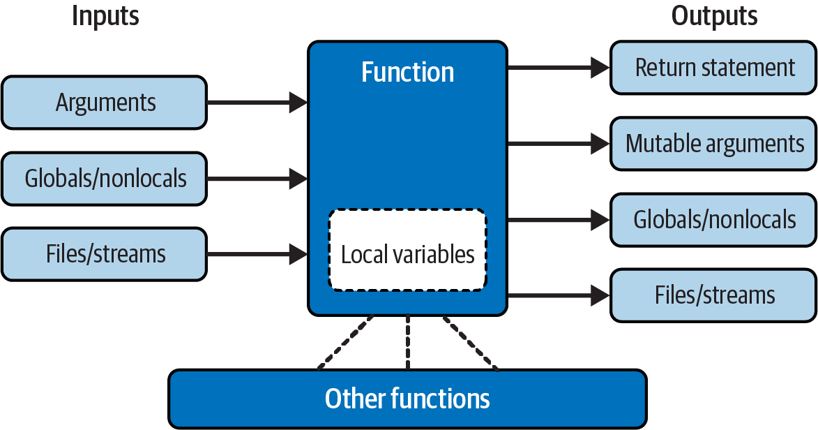
Figure 19-1. Function execution environment
Of course, there are plenty of exceptions to the preceding design rules, including some related to Python’s OOP support. As you’ll see in Part VI, Python classes depend on changing a passed-in mutable object—class functions set attributes of an automatically passed-in argument called self to change per-object state information (e.g., self.edition=6). Moreover, if classes are not used, global variables are a straightforward way for functions in modules to retain single-copy state between calls. Side effects are usually dangerous only if they’re unexpected.
In general though, you should strive to minimize external dependencies in functions and other program components. The more self-contained a function is, the easier it will be to understand, reuse, and modify. Making code as freestanding as possible is especially important when functions go multilevel with recursion, per the next section.
Recursive Functions
We mentioned recursion in relation to comparisons of core types in Chapter 9. While discussing scope rules near the start of Chapter 17, we also briefly noted that Python supports recursive functions—functions that call themselves either directly or indirectly in order to loop. In this section, we’ll explore what this looks like in our functions’ code.
Recursion is a somewhat advanced topic, and it’s relatively uncommon to see in Python, partly because Python’s procedural shed includes simpler looping tools. Still, it’s a useful technique to know about, as it allows programs to traverse structures that have arbitrary and unpredictable shapes and depths—planning travel routes, analyzing language, and crawling links on the Web, for example. Recursion is even an alternative to simple loops and iterations, though not necessarily the simplest or most efficient one.
Summation with Recursion
Let’s turn to some examples. To sum a list (or other sequence) of numbers, we can either use the built-in sum function or write a more custom version of our own. Example 19-1 shows what a custom summing function might look like when coded with recursion.
Example 19-1. mysum.py
def mysum(L):
    if not L:
        return 0
    else:
        return L[0] + mysum(L[1:])       # Call myself recursively
To use, either add self-test code to the bottom of this file and run it as a script, or import it as a module and test at the REPL (again, the file may need to be in the folder where you’re working either way, per Chapter 3). With the latter:
>>>from mysum import mysum# Import file as a module in a REPL>>>mysum([1, 2, 3, 4, 5])# Sum all the numbers in any sequence15
At each level, this function calls itself recursively to compute the sum of the rest of the list, which is later added to the item at the front. This recursive loop ends and zero is returned when the list becomes empty. When using recursion like this, each open level of call to the function has its own copy of the function’s local scope on the runtime call stack. Here, that means L is different in each level, so each remembers its own segment of the list.
If this is difficult to understand (and it often is for new programmers), try adding a print of L to the function and run it again, to trace the current list at each call level; here’s the required mod pasted at the REPL for variety:
>>>def mysum(L): print(L)# Trace recursive levelsif not L:# L shorter at each levelreturn 0 else: return L[0] + mysum(L[1:])>>>mysum([1, 2, 3, 4, 5])[1, 2, 3, 4, 5] [2, 3, 4, 5] [3, 4, 5] [4, 5] [5] [] 15
As you can see, the list to be summed grows smaller at each recursive level, until it becomes empty—the termination of the recursive loop. The sum is then computed as the recursive calls unwind on returns.
Coding Alternatives
Interestingly, we can use Python’s if/else ternary expression (described in Chapter 12) to save some code real estate here. We can also generalize for any summable type (which is easier if we assume at least one item in the input) and use extended unpacking assignment to make the first/rest unpacking simpler (as covered in Chapter 11). Example 19-2 collects all three of these mods, ready to be run in a file or pasted into a REPL.
Example 19-2. mysum_alts.py
def mysum(L):
    return 0 if not L else L[0] + mysum(L[1:])           # Use ternary expression

def mysum(L):
    return L[0] if len(L) == 1 else L[0] + mysum(L[1:])  # Any type, assume one+

def mysum(L):
    first, *rest = L
    return first if not rest else first + mysum(rest)    # Use extended unpacking
When tested individually, all three of these alternatives handle numeric summation the same as the original:
>>> mysum([1, 2, 3, 4, 5])
15
Uniquely, the latter two fail for empties (e.g., mysum([])), but handle sequences of any object type that supports +, not just numbers (for strings, the effect is similar to ''.join(L)):
>>>mysum(('h', 'a', 'c', 'k'))# The last two fail on mysum([])'hack' >>>mysum(['hack', 'app', 'code'])# But they support nonnumeric types'hackappcode'
Run some tests on your own for more insight. If you study these three variants, you’ll also find that:
The latter two work on a single string argument (e.g.,
mysum('hack')), because strings are sequences of one-character strings (though this use case isn’t very useful: you get back the same string).The third variant also works on arbitrary iterables, including open input files (
mysum(open(name))), but the others’ indexing generally fails on nonsequences (see Chapter 14 for extended unpacking demos).
You may also notice that the third variant’s unpacking assignment is similar to a * collector in a function header, and it’s tempting to recode it as such. This won’t quite work, though, because it would expect individual arguments, not a single iterable—unless we also star both the top-level input and recursive call. Here’s the end result, though by summing discrete arguments, it solves a different problem than both the prior versions and built-in sum:
>>>def mysum(first, *rest):return first if not rest else first + mysum(*rest)>>>mysum(*[1, 2, 3, 4, 5])15 >>>mysum(*'hack')'hack'
Finally, bear in mind that recursion can be either direct, as in the examples so far, or indirect, as in the following—a function that calls another function, which calls back to its caller. The net effect is the same, though there are two function calls at each level instead of one:
>>>def mysum(L): if not L: return 0 return nonempty(L)# Call a function that calls me>>>def nonempty(L): return L[0] + mysum(L[1:])# Indirectly recursive>>>mysum([1.1, 2.2, 3.3, 4.4])11.0
Loop Statements Versus Recursion
Though recursion works for summing in the prior sections’ examples, it’s probably overkill in this context. In fact, recursion is not used nearly as often in Python as in more esoteric languages like Prolog or Lisp, because Python emphasizes simpler procedural statements like loops, which are usually more natural. The while, for example, often makes things more concrete, and it doesn’t require that a function be defined to allow recursive calls:
>>>L = [1, 2, 3, 4, 5]>>>tot = 0>>>while L:tot += L[0]L = L[1:]>>>tot15
Better yet, for loops iterate for us automatically, making recursion largely extraneous in many cases (and, in all likelihood, less efficient in terms of memory space and execution time):
>>>L = [1, 2, 3, 4, 5]>>>tot = 0>>>for x in L: tot += x>>>tot15
With looping statements, we don’t require a fresh copy of a local scope on the call stack for each iteration, and we avoid the speed costs associated with function calls in general. (Stay tuned for Chapter 21’s timer case study for ways to compare the execution times of alternatives like these.)
Handling Arbitrary Structures
On the other hand, recursion—or equivalent and explicit stack-based algorithms we’ll explore shortly—can be required to traverse arbitrarily shaped structures. As a simple example of recursion’s role in this context, consider the task of computing the sum of all the numbers in a nested sublists structure like this:
[1, [2, [3, 4], 5], 6, [7, 8]] # Arbitrarily nested sublists
Neither our prior summers nor simple looping statements will work here because this is not a linear iteration. Nested looping statements do not suffice either—because the sublists may be nested to arbitrary depth and in an arbitrary shape, there’s no way to know how many nested loops to code to handle all cases. Instead, the function in Example 19-3 accommodates such general nesting by using recursion to visit sublists along the way.
Example 19-3. sumtree.py
def sumtree(L, trace=False):
    tot = 0
    for x in L:                                 # For each item at this level
        if not isinstance(x, list):
            tot += x                            # Add numbers directly
            if trace: print(x, end=', ')
        else:
            tot += sumtree(x, trace)            # Recur for sublists
    return tot
In this file’s function, each recursive level runs a for loop to add numbers, or recur into sublists to open new levels. Recall from Chapter 9 that isinstance compares object types; it’s used here to detect nested sublists.
This code is also instrumented to trace items as they are added to the total: if trace is passed a true value, you can see how the object is scanned left to right. Because it also steps down into sublists with recursion along the way, though, the traversal is really both horizontal and vertical:
>>>from sumtree import sumtree>>>sumtree([1, [2, [3, 4], 5], 6, [7, 8]])36 >>>sumtree([1, [2, [3, 4], 5], 6, [7, 8]], trace=True)1, 2, 3, 4, 5, 6, 7, 8, 36
Testing with a separate script
At this point, we could test other cases by typing them interactively or by adding code to the bottom of the file, but you’re probably starting to see that this can be a bit limiting. Instead, the script in Example 19-4 makes the process automatic and easily repeatable. As a bonus, it can be used for other summers we’ll code in a moment.
Example 19-4. sumtree_tester.py
tests = ( [1, [2, [3, 4], 5], 6, [7, 8]],# Mixed nesting => 36[1, [2, [3, [4, [5]]]]],# Right-heavy nesting => 15[[[[[1], 2], 3], 4], 5])# Left-heavy nesting => 15def tester(sumtree, trace=True): for test in tests: print(sumtree(test, trace))
To use this tester, simply import both summer and tester, and pass the former to the latter. When run, our summer prints numbers as added with the final sum at the end, for each of three canned tests:
>>>from sumtree import sumtree# Get the summer>>>from sumtree_tester import tester# Get the tester>>>tester(sumtree)# Run the tester on the summer1, 2, 3, 4, 5, 6, 7, 8, 36 1, 2, 3, 4, 5, 15 1, 2, 3, 4, 5, 15
Within tester, sumtree refers to the summer function passed into it. Again, because functions are objects, passing them around this way is natural, and makes code flexible.
Recursion versus queues and stacks
It sometimes helps recursion newcomers to understand that internally, Python implements recursion by pushing information on a call stack at each recursive call, so it remembers where it must return and continue later. In fact, it’s generally possible to implement recursive-style procedures without recursive calls, by using an explicit stack or queue of your own to keep track of remaining steps.
For instance, Example 19-5 computes the same sums as the prior example, but uses an explicit list to schedule when it will visit items in the subject, instead of issuing recursive calls. The item at the front of the list is always the next to be processed and summed.
Example 19-5. sumtree_queue.py
def sumtree(L, trace=False):# Breadth-first, explicit queuetot = 0 items = list(L)# Start with copy of top levelwhile items: front = items.pop(0)# Fetch/delete front itemif not isinstance(front, list): tot += front# Add numbers directlyif trace: print(front, end=', ') else: items.extend(front)# <== Append all in nested listreturn tot
Technically, this code traverses the list in breadth-first fashion (across before down), because it adds nested lists’ contents to the end of the list—forming a FIFO (first-in-first-out) queue. The net effect sums by horizontal levels. To test, we can either import and use the new summer directly, or route it to the Example 19-4 tester to be exercised automatically with tracing:
>>>from sumtree_queue import sumtree# Get the new summer>>>sumtree([1, [2, [3, 4], 5], 6, [7, 8]])36 >>>from sumtree_tester import tester# Unless already imported>>>tester(sumtree)# Run tester on _this_ summer1, 6, 2, 5, 7, 8, 3, 4, 36 1, 2, 3, 4, 5, 15 5, 4, 3, 2, 1, 15
Fine points: we don’t have to reimport the tester again if it’s already been imported in this session, and importing the same-named summer just works—the new summer’s filename makes it unique, and sumtree is always the latest version imported if you import more than one, because imports assign names (see Chapter 18’s print emulators for another example of this pattern at work, and watch for more on imports in this book’s next part).
More importantly, notice how the order in which numbers visited here is different than in the original recursive-call version, due to the breadth-first queue. Trace through the tester’s tests to see how this pans out.
If we instead want to emulate the traversal of the recursive-call version more closely, we can change this code to perform depth-first traversal (down before across) simply by adding the contents of nested lists to the front of the list—forming a last-in-first-out (LIFO) stack. Example 19-6 makes the required mods, but the only way it differs from the breadth-first version is the line that adds to the front instead of the end, marked with <== in a comment.
Example 19-6. sumtree_stack.py
def sumtree(L, trace=False):# Depth-first, explicit stacktot = 0 items = list(L)# Start with copy of top levelwhile items: front = items.pop(0)# Fetch/delete front itemif not isinstance(front, list): tot += front# Add numbers directlyif trace: print(front, end=', ') else: items[:0] = front# <== Prepend all in nested listreturn tot
As before, we can use this function directly, or pass it to the same tester; its file makes it distinct, and its name refers to the latest import. When run, this summer visits numbers in the same order as the recursive-calls original, but manages the traversal with an explicit stack instead of recursion:
>>>from sumtree_stack import sumtree# Same name, different file>>>sumtree([1, [2, [3, 4], 5], 6, [7, 8]])36 >>>from sumtree_tester import tester# Optional if already imported>>>tester(sumtree)1, 2, 3, 4, 5, 6, 7, 8, 36 1, 2, 3, 4, 5, 15 1, 2, 3, 4, 5, 15
For more on the last two examples (plus another breadth-first coding variant omitted here), see file sumtree_etc.py in the book’s examples package. It adds additional tracing so you can watch it walk structures in more detail.
In general, though, once you get the hang of recursive calls, they may be more natural than the explicit scheduling lists they automate, and are generally preferred unless you need to traverse structures in specialized ways. Some programs, for example, perform a best-first search that requires an explicit search queue ordered by relevance or other criteria. If you think of a web crawler that scores sites visited by content, the applications may start to become clearer.
Cycles, paths, and stack limits
As is, these programs suffice as demos, but larger recursive applications can sometimes require a bit more infrastructure than shown here: they may need to avoid cycles or repeats, record paths taken for later use, and expand stack space when using recursive calls instead of explicit queues or stacks.
For instance, neither the recursive-call nor the explicit queue/stack examples in this section do anything about avoiding cycles—visiting a location already visited. That’s not required here, because we’re traversing strictly hierarchical trees of list objects. If data can be a cyclic graph, though, both these schemes will fail: the recursive-call scheme will fall into an infinite recursive loop (and may run out of call-stack space), and the others will fall into simple infinite loops, re-adding the same items to their lists (and may or may not run out of general memory). In fact, it’s easy to demo the perils by creating a cyclic object with the strange code we met in an exercise at the end of Chapter 3:
>>>L = [1, 2]>>>L.append(L)# Make a cyclic object: L references itself>>>L[1, 2, [...]] >>>from sumtree import sumtree>>>sumtree(L)RecursionError: maximum recursion depth exceeded >>>from sumtree_queue import sumtree>>>sumtree(L)…hang or crash, and ditto for stack…
Some programs also need to avoid repeated processing for a state reached more than once, even if that wouldn’t lead to a loop. To do better, a recursive-call traversal might make and pass along a mutable set, dictionary, or list of states visited so far and check for repeats as it goes. We will use this scheme in later recursive examples in this book:
  if state not in visited:
      visited.add(state)          # x.add(state), x[state]=True, or x.append(state)
      …proceed…
Nonrecursive alternatives might similarly avoid adding states already visited with code like the following. Subtly, object cycles may require is (not in), and simply checking for duplicates already on the items list would avoid scheduling a state twice but would not prevent revisiting a state visited earlier and hence removed from that list:
  visited.add(front)
  …proceed…
  items.extend([x for x in front if x not in visited])
This model doesn’t quite apply to this section’s use case that simply adds numbers in lists, but other applications will generally be able to identify repeated states—a URL of a previously visited web page, for instance. In fact, we’ll use such techniques to avoid cycles and repeats in the later examples listed in the next section.
Some programs may also need to record complete paths for each state followed so they can report solutions when finished. In such cases, each item in the nonrecursive scheme’s stack or queue may be a full path list that suffices for a record of states visited, and contains the next item to explore at either end.
Also note that standard Python limits the depth of its runtime call stack—crucial to recursive-call programs—to trap infinite recursion errors. To expand it for deeper journeys, use the sys module:
>>>sys.getrecursionlimit()# 1000 calls deep default1000 >>>sys.setrecursionlimit(10000)# Allow deeper nesting>>>help(sys.setrecursionlimit)# Read more about it
The maximum allowed setting can vary per platform. This isn’t required for programs that use stacks or queues to avoid recursive calls and gain more control over the traversal process (though they also won’t catch infinite loops).
More recursion examples
Although this section’s example is artificial, it is representative of a larger class of programs; inheritance trees and module import chains, for example, can exhibit similarly general structures, and computing tools such as permutations can require arbitrarily many nested loops. In fact, we’ll use recursion again in such roles later in this book:
In Chapter 20’s permute.py, to shuffle arbitrary sequences
In Chapter 25’s reloadall.py, to traverse import chains
In Chapter 29’s classtree.py, to traverse class inheritance trees
In Chapter 31’s lister.py, to traverse class inheritance trees again
In Appendix B, “Solutions to End-of-Part Exercises” at the end of this part of the book: countdowns and factorials
The second and third of these will also detect states already visited to avoid cycles and repeats. Although simple loops should generally be preferred to recursion for linear iterations on the grounds of simplicity and efficiency, you’ll find that recursion is essential in scenarios like those in these later examples.
Moreover, you sometimes need to be aware of the potential of unintended recursion in your programs. As you’ll also see later in the book, some operator-overloading methods in classes such as __setattr__ and __getattribute__ and even __repr__ have the potential to recursively loop if used incorrectly. Recursion is a powerful tool, but it tends to be best when both understood and expected!
Function Tools: Attributes, Annotations, Etc.
Let’s move on to a category of tools that may seem less ethereal than recursion to some earthlings. As we’ve seen in this part of the book, functions in Python are much more than code-generation specifications for a compiler—they are full-blown objects, stored in pieces of memory all their own. As such, they can be freely passed around a program and called indirectly. They also support operations that have little to do with calls at all, including attributes and annotation. We’ve sampled some of these topics earlier, but this section provides expanded coverage.
The First-Class Object Model
Because Python functions are objects, you can write programs that process them generically. Function objects may be reassigned to other names, passed to other functions, embedded in data structures, returned from one function to another, and more, as if they were simple numbers or strings. Function objects happen to support a special operation—they can be called by listing arguments in parentheses—but they belong to the same general category as other objects.
As we’ve seen, this is usually called a first-class object model; it’s ubiquitous in Python, and a necessary part of functional programming. We’ll explore this programming mode more fully in this and the next chapter; because its motif is founded on the notion of applying functions, it treats functions as a kind of data.
We’ve explored some generic use cases for functions in earlier examples, but a quick review helps to underscore the model. For example, there’s really nothing special about the name used in a def statement: it’s just a variable assigned in the current scope, as if it had appeared on the left of an = sign. Because the function name is simply a reference to an object after a def runs, you can reassign that object to other names freely and call it through any reference:
>>>def exclaim(message):# Name exclaim assigned to function objectprint(message + '!')>>>exclaim('Direct call')# Call object through original nameDirect call! >>>x = exclaim# Now x references the function too>>>x('Indirect call')# Call object through name x by adding ()Indirect call!
And because arguments are passed by assigning objects, it’s just as easy to pass functions to other functions as arguments. The callee may then call the passed-in function just by adding arguments in parentheses (see the earlier summer tester in Example 19-4 for another example of this pattern):
>>>def generic(func, arg): func(arg)# Call the passed-in object by adding ()>>>generic(exclaim, 'Argument call')# Pass the function to another functionArgument call!
You can even stuff function objects into data structures, as though they were integers or strings. The following, for example, embeds the function twice in a list of tuples, as a sort of actions table. Because Python compound types like these can contain any sort of object, there’s no special case here, either (Example 18-2 used similar code):
>>>schedule = [ (exclaim, 'Hack'), (exclaim, 'Code') ]>>>for (func, arg) in schedule: func(arg)# Call functions embedded in containersHack! Code!
This code simply steps through the schedule list, calling the exclaim function with one argument each time through. As we saw in Chapter 17’s examples, functions can also be created and returned for use elsewhere—the closure created in this mode also retains state from the enclosing scope:
>>>def implore(verb):# Make a function but don't call itdef exclaim(noun): print(f'{verb} {noun}!') return exclaim>>>I = implore('Hack')# Label in enclosing scope is retained>>>I('Code')# Call the function that make returnedHack Code! >>>I('App')Hack App!
Python’s first-class object model and lack of type constraints make for a very flexible programming language.
Function Introspection
In fact, functions are more flexible than you might expect. Because they are objects, we can also process functions with normal object tools. For instance, by now we know that once we make a function we can call it as usual:
>>>def func(a): b = 'Hack' return b * a>>>func(8)'HackHackHackHackHackHackHackHack'
But the call expression is just one of a set of operations defined to work on function objects. For instance, we can also inspect their attributes generically:
>>>func.__name__'func' >>>dir(func)'__annotations__', '__builtins__', '__call__', '__class__', '__closure__', …more omitted: 38 total… '__setattr__', '__sizeof__', '__str__', '__subclasshook__', '__type_params__']
Introspection—internals access—tools like this allow us to explore implementation details. For example, functions have attached code objects, which provide details on aspects such as the functions’ local variables and arguments:
>>>func.__code__<code object func at 0x103ef3910, file "<stdin>", line 1> >>>dir(func.__code__)['__class__', '__delattr__', '__dir__', '__doc__', '__eq__', '__format__', '__ge__', …more omitted: 48 total… 'co_posonlyargcount', 'co_qualname', 'co_stacksize', 'co_varnames', 'replace'] >>>func.__code__.co_varnames('a', 'b') >>>func.__code__.co_argcount1
Tool writers can make use of such information to manage functions—in fact, we will too in the online-only “Decorators” chapter, to implement validation of function arguments with the decorators introduced ahead. Whether you code or use such tools, object introspection boosts function utility.
Function Attributes
Nor are function objects limited to the system-defined attributes of the prior section: it’s also possible to attach arbitrary user-defined attributes to them. This topic was introduced in Chapter 17, but this section expands on it with additional context and examples. As usual in Python, function attributes are created by simple assignments:
>>>def func(): pass>>>func<function func at 0x1043771a0> >>>func.count = 0>>>func.count += 1>>>func.count1 >>>func.handles = 'Button-Press'>>>func.handles'Button-Press' >>>dir(func)…most double-underscore names omitted… '__str__', '__subclasshook__', '__type_params__', 'count', 'handles']
Python’s own implementation-related data stored on functions follows naming conventions that prevent them from clashing with the more arbitrary attribute names you might assign yourself. Specifically, all function internals’ names have leading and trailing double underscores (“__X__”):
>>>len(dir(func))40 >>>[x for x in dir(func) if not x.startswith('__')]['count', 'handles']
If you’re careful not to name attributes the same way as Python, you can safely use the function’s namespace as though it were your own namespace or scope. Naturally, all of this works the same for functions made with lambda:
>>>F = lambda: None>>>len(dir(F))38 >>>F.book = 'LP6E'>>>F.book'LP6E'
As covered in Chapter 17, such attributes can be used to attach state information to function objects directly, instead of using other techniques such as globals, nonlocals, and classes. Unlike nonlocals, such attributes are accessible anywhere the function itself is, even from outside its code.
In a sense, this is also a way to emulate “static locals” in other languages—variables whose names are local to a function, but whose values are retained after a function exits. Attributes are related to objects instead of scopes (and must be referenced through the function name within its code), but the net effect is similar.
Moreover, as also explored in Chapter 17, when attributes are attached to functions generated by other factory functions, they also support multiple copy, writeable, and per-call state retention, as an alternative to closures and class-instance attributes. This makes function attributes a broadly useful tool—like the topics of the next section.
Function Annotations and Decorations
For tools roles, functions also support attached annotations—arbitrary user-defined info about a function’s arguments and result that augment the function. Python provides syntax for coding annotations, but it doesn’t do anything with them itself—annotations are completely optional, don’t impact function behavior in any way, and when present are simply attached to the function object’s __annotations__ attribute for use by other tools.
While not of general interest to most application programmers, third-party tools and libraries might use annotations in the context of enhanced error checking, or API directives. Type hinting, discussed in Chapter 6, is also based on annotations, but is optional and unused, and doesn’t preclude other roles for annotations today (more on this ahead).
We studied the formal rules for arguments in function definitions in the preceding chapter. Annotations don’t modify these rules but simply extend their syntax to allow extra expressions to be associated with named arguments and function results. Consider the following nonannotated function, coded with three arguments and a returned result:
>>>def func(a, b, c): return a + b + c>>>func(1, 2, 3)6
Syntactically, function annotations are coded in def header lines (only), as arbitrary expressions associated with arguments and return values. For arguments, they appear after a colon immediately following the argument’s name; for return values, they are written after a -> following the arguments list’s closing parenthesis. The following code, for example, annotates all three of the prior function’s arguments, as well as its return value:
>>>def func(a: 'hack', b: (1, 10), c: float) -> int: return a + b + c>>>func(1, 2, 3)6
Calls to an annotated function work as usual, but when annotations are present Python collects them in a dictionary and attaches it to the function object itself as its __annotations__. In this, argument names become keys; the return value annotation is stored under key return if coded (which suffices because this reserved word can’t be used as an argument name); and the values of annotation keys are assigned to the results of the annotation expressions:
>>> func.__annotations__
{'a': 'hack', 'b': (1, 10), 'c': <class 'float'>, 'return': <class 'int'>}
Because they are just Python objects attached to a Python object, annotations are straightforward to process. The following annotates just two of three arguments and steps through the attached annotations generically:
>>>def func(a: 'python', b, c: 3.12): return a + b + c>>>func(1, 2, 3)6 >>>func.__annotations__{'a': 'python', 'c': 3.12} >>>for arg in func.__annotations__: print(arg, '=>', func.__annotations__[arg])a => python c => 3.12
There are two fine points to note here. First, you can still use defaults for arguments if you code annotations—the annotation (and its : character) appear before the default (and its = character). In the following, for example, a: 'hack' = 4 means that argument a defaults to 4 and is annotated with the string 'hack':
>>>def func(a: 'hack' = 4, b: (1, 10) = 5, c: float = 6) -> int: return a + b + c>>>func(1, 2, 3)# No defaults used6 >>>func()# a=4 + b=5 + c=6 (all defaults)15 >>>func(1, c=10)# 1 + b=5 + 10 (keywords work normally)16 >>>func.__annotations__{'a': 'hack', 'b': (1, 10), 'c': <class 'float'>, 'return': <class 'int'>}
Second, note that the blank spaces in the prior example are all optional—you can use spaces between components in function headers or not, but omitting them might degrade your code’s readability to some observers (and probably improve it to others):
>>>def func(a:'hack'=4, b:(1,10)=5, c:float=6)->int: return a + b + c>>>func(1, 2)# 1 + 2 + c=69 >>>func.__annotations__{'a': 'hack', 'b': (1, 10), 'c': <class 'float'>, 'return': <class 'int'>}
While annotations are optional and uncommon, they may be used to specify constraints for types or values, and larger APIs might use this feature as a way to register function interface information. In fact, you’ll see a potential application in the online-only “Decorators” chapter, when we code annotations as an alternative to function decorator arguments—a more general concept in which augmentation info is coded outside the function header and so is not limited to a single role.
Function decorators alternative: Preview
Because we’re going to devote an entire chapter to decorators, we’ll omit most of their story here. But as a very brief preview, decorators are simply functions that augment other functions. They are applied to another function’s def with an @ prefix that rebinds the other function’s name to the result of passing it to the decorator. This syntax:
@decorator
def func(args): …           # Decorated function def
is automatically morphed into the following equivalent, where decorator is a one-argument callable object (or an expression that returns one), which returns a callable object having arguments compatible with func (or func itself):
def func(args): …
func = decorator(func)      # Rebind func to decorator's result
Decorators can use this hook to wrap another function in an extra layer of code for nearly arbitrary purposes, as in the following code the adds a message when a decorated function is called:
def echo(F):
    def proxy(*args):
        print('calling', F.__name__)       # Add actions here
        return F(*args)                    # Run decorated function
    return proxy

@echo
def func(x, y):                            # Rebinds func = echo(func)
    print('I am running...', x, y)         # func is run by the proxy closure

>>> func(1, 2)                             # Runs a proxy, which runs func
calling func
I am running... 1 2
As you’ll learn later, decorators can also take arguments (e.g., @echo(args)) whose utility can overlap with annotations—argument info can be sent to the decorator instead of being embedded in headers as annotations. Because this is an advanced tool that can also be applied to classes, we’ll pause this thread until Chapter 32 and the online-only “Decorators” chapter.
Compared to annotations, though, decorators don’t complicate function headers themselves with extra syntax, and more naturally support multiple roles. Annotations may make functions difficult to read, and generally can have just one role—one that’s hijacked by the optional type hinting of Chapter 6 in programs that choose to employ it.
In fact, type hinting advocates have tried to deprecate all other roles for annotations. While these divisive (and perhaps even rude) efforts have thankfully failed to date, decorators face no such challenge, and may be a safer bet going forward. Today, though, both annotations and decorations are tools whose roles are limited only by your imagination.
Finally, note that annotations and decorations work in def statements—but not in lambda expressions, whose syntax by design limits the functions they can define. Coincidentally, this brings us to this potpourri’s next topic.
Anonymous Functions: lambda
We first met the lambda expression back in Chapter 16 and have used it in a handful of examples since then. This section reviews the basics and takes a deeper second look, to both reinforce and expand on this topic.
As we’ve seen, besides the def statement, Python provides an expression that creates function objects. Because of its similarity to a tool in other languages, it’s called lambda. Like def, this expression creates a function to be called later, but it returns the function instead of assigning it to a name. This is why lambdas are sometimes known as anonymous functions. In practice, they are used to inline function definitions, or defer execution of code.
Note
What’s in a name?: The lambda tends to intimidate people, largely due to the name “lambda” itself—a name that comes from the Lisp language, which got it from lambda calculus, which is a form of symbolic logic. Obscure mathematical heritage aside, though, lambda in Python is really just a word that introduces an expression syntactically, and its expression is simply an alternative way to code a function—albeit without statements, decorators, or annotations.
lambda Basics
As a refresher, the lambda’s general form is the keyword lambda, followed by zero or more arguments (just like the arguments you enclose in parentheses in a def header, sans annotations), followed by an expression after a colon:
lambdaargument1,argument2,…argumentN:expression-using-arguments
Parentheses are not allowed around lambda arguments and are generally optional around the entire lambda itself, though they’re required in some contexts and may boost clarity in others. Functions returned by lambda work the same as those assigned by def, but lambda differs in ways that make it useful in specialized roles:
lambdais an expression, not a statement. Because of this, alambdacan appear in places adefis not allowed by Python’s syntax—inside a list literal or a function call’s arguments, for example. Withdef, functions can be referenced by name in such locations, but must be created elsewhere. As an expression,lambdareturns a value (a new function) that can be assigned a name, or used where thelambdaappears.lambda’s body is a single expression, not a block of statements. Thelambda’s body is similar to what you’d put in adefbody’sreturnstatement; you simply type the result as a naked expression, instead of explicitly returning it. Because it is limited to an expression, alambdais less general than adef—you can only squeeze so much logic into alambdabody without full-blown statements. This is by design, to limit program nesting:lambdais designed for coding simple functions, anddefhandles larger tasks.
Apart from those distinctions, defs and lambdas do the same sort of work. For instance, by this point we should be pros at making a function with a def statement:
>>>def func(x, y, z): return x + y + z>>>func(2, 3, 4)9
But we can achieve the same effect with a lambda expression by explicitly assigning its result to a name through which you can later call the otherwise-anonymous function:
>>>func = lambda x, y, z: x + y + z>>>func(2, 3, 4)9
Here, func is manually assigned the function object the lambda expression creates; this is how def works, too, but its assignment is automatic. Defaults and other argument-matching syntax work in lambda too, just like in a def:
>>>x = (lambda a='hack', b='python', c='code': a + b + c)>>>x('write')'writepythoncode'
The code in a lambda body also follows the same scope lookup rules as code inside a def. lambda expressions introduce a new local scope much like a nested def, which automatically sees names in enclosing functions, the module, and the built-in scope—via the LEGB rule we studied in Chapter 17:
>>>def editions(title):# title in enclosing scope return (lambda e: title + ', ' + e)# Return a function object>>>labeler = editions('Learning Python')# Make+save nested function>>>labeler('6E')# '6E' passed to e in lambda'Learning Python, 6E'
With those basic lambda “hows” in hand, the natural next question is “why,” taken up in the next section.
Why Use lambda?
Generally speaking, lambda is a sort of function shorthand that allows you to embed a function’s definition within the code that uses it. It is entirely optional—you can always use def instead, and should if your function requires the power of full statements that the lambda’s expression cannot provide. But lambda may be easier to use in scenarios where you just need to embed a small bit of executable code inline at the place where it is to be later used.
For instance, you’ll see later that callback handlers are frequently coded as inline lambda expressions embedded directly in a registration call’s arguments list, instead of being defined with a def elsewhere in a file and referenced by name (see the sidebar “Why You Will Care: lambda Callbacks” for an example).
lambda is also commonly used to code jump tables, which are lists or dictionaries of actions to be performed on demand. For example:
L = [lambda x: x * 2,# Inline function definitionlambda x: x ** 2, lambda x: x // 2]# A list of three callable functionsfor f in L: print(f(5))# Prints 10, 25, and 2print(L[1](5))# Prints 25
The lambda expression works well when you need to stuff small pieces of executable code into places where statements like def are not allowed. The preceding code snippet, for example, builds up a list of three functions by embedding lambda expressions inside a list literal; a def won’t work inside a literal like this because it is a statement, not an expression. The equivalent def coding would require temporary function names (which might clash with others) and function definitions outside the context of intended use (which might be hundreds of lines away):
def f1(x): return x * 2 def f2(x): return x ** 2# Define named functionsdef f3(x): return x // 4# Separate from their place of useL = [f1, f2, f3]# Reference by namefor f in L: print(f(2))# Also prints 10, 25, and 2
Multiway branches: The finale
In fact, you can do the same sort of thing with dictionaries and other data structures in Python to build up more general sorts of action tables. Here’s another example to illustrate at the interactive prompt:
>>>key = 'loop'>>>{'hack': lambda s: s.upper(), 'code': lambda s: s.lower(), 'loop': lambda s: f'{s * 4}!'}[key]('Py')'PyPyPyPy!'
Here, when Python makes the temporary dictionary, each of the nested lambdas generates and leaves behind a function to be called later. Indexing by key fetches one of those functions, and parentheses force the fetched function to be called. When coded this way, a dictionary becomes a more general multiway branching tool than this book could fully reveal in Chapter 12’s coverage of if statements.
To make this work without lambda, you’d need to instead code three def statements somewhere else in your file, outside the dictionary in which the functions are to be used, and reference the functions by name:
>>>def f1(s): return s.upper()>>>def f2(s): return s.lower()>>>def f3(s): return f'{s * 4}!'>>>key = 'loop'>>>{'hack': f1, 'code': f2, 'loop': f3}[key]('Py')'PyPyPyPy!'
This works, too, but your defs may be arbitrarily far away in your file, even if they are just little bits of code. The code proximity that lambda provides is especially useful for functions that will only be used in a single context—if the three functions here are not useful anywhere else, it makes sense to embed their definitions within the dictionary as lambdas. Moreover, the def form requires you to make up names for these little functions that, again, may clash with other names in this file (perhaps unlikely, but always possible).1
You can use the match statement today with similar results, but it may require even more code than def scheme, especially since you’d have to nest it within a def to support an argument like s; see Chapter 12 for more info. lambda is also handy in function-call argument lists as a way to inline temporary function definitions not used anywhere else in your program; you’ll see examples of such other uses later in this chapter, when we study map.
Note
The siren song of eval: In principle, you could skip the dispatch table in the preceding code if the function name is the same as its string lookup key—an eval(key)(arg) would kick off the call. While true in this case and sometimes useful, as we saw earlier (e.g., Chapter 10), eval is relatively slow (it must compile and run code), and insecure (you must trust the string’s source). More fundamentally, jump tables are generally subsumed by polymorphic method dispatch in Python: calling a method does the “right thing” based on the type of object that’s the subject of the call, no switching logic required. To see why, stay tuned for Part VI.
How (Not) to Obfuscate Your Python Code
The fact that the body of a lambda has to be a single expression (not a series of statements) would seem to place severe limits on how much logic you can pack into a lambda. If you know what you’re doing, though, you can code most statements in Python as expression-based equivalents.
For example, if you want to print from the body of a lambda function, simply use print or sys.stdout.write (recall from Chapter 11 that this is what print really does). And to execute multiple actions, code a sequence like a tuple, to evaluate nested multiple expressions from left to right (tuples require parentheses in this context):
>>>series = lambda a, b: (print(a.upper()), print(b.lower()))# > 1 actions>>>ignore = series('Hack', 'Code')HACK code
Similarly, to nest logic in a lambda, you can use the if/else ternary expression introduced in Chapter 12, or the equivalent but trickier and/or combination also described there. As you learned earlier, the following statement:
if a:
    b
else:
    c
can be emulated by either of these equivalent expressions (the second is only roughly the same, but close enough):
b if a else c
((a and b) or c)
Because expressions like these can be placed inside a lambda, they may be used to implement selection logic within a lambda function (the lambda is parenthesized here only for variety and subjective clarity):
>>>lower = (lambda x, y: x if x < y else y)# Ifs in lambda: ternary>>>lower('bb', 'aa')'aa' >>>lower('aa', 'bb')'aa'
Furthermore, if you need to perform loops within a lambda, you can also embed things like list comprehension expressions and map calls—tools we met in earlier chapters and will revisit in this and the next chapter:
>>>showall = lambda x: [print(y) for y in x]# Loops in lambda: list comp>>>t = showall(['lp5e', 'lp6e'])lp5e lp6e >>>showall = lambda x: list(map(print, x))# Loops in lambda: maps>>>t = showall(('py3.3', 'py3.12'))py3.3 py3.12 >>>showall = lambda x: print(*x, sep='', end='')# Another option: *unpacking
And while it’s limited by the local scope of the function that lambda makes, assignment is in scope (pun intended) for lambda expressions that use the := named-assignment expression:
>>>namer = lambda x: (res := x + 1) + res# Assignment in lambda: :=>>>namer(2)6 >>>res# But it doesn't persistNameError: name 'res' is not defined
There is a limit to emulating statements with expressions: you can’t assign nonlocals, for instance, though tools like the setattr built-in, the __dict__ of namespaces, and methods that change mutable objects in place can sometimes stand in—and can quickly lead you deep into the heart of expression-convolution darkness.
But now that this book has shown you these tricks, it must also humbly implore you to use them only as a last resort. Without due care, they can yield unreadable (a.k.a. obfuscated) Python code, despite the language’s best intents. In general, simple is better than complex, explicit is better than implicit, and full statements are better than arcane expressions. That’s why lambda is limited to expressions. If you have larger logic to code, use def; lambda is for small pieces of inline code. On the other hand, you may find these techniques useful—when taken in moderation.
Scopes: lambdas Can Be Nested Too
One last lambda note: as we saw in Chapter 17, lambda is also the main beneficiary of enclosing-function scope lookup—the E in the LEGB scope rule. As a review, in the following the lambda appears inside a def, its typical coding, and so can access the value that name x had in the enclosing function’s scope during its call:
>>>def action(x): return (lambda y: x + y)# Make function, remember x>>>act = action(99)>>>act(2)# Call what action returned101
What wasn’t illustrated in the prior discussion of nested function scopes is that a lambda also has access to the names in any enclosing lambda. This case is somewhat obscure, but imagine if we recoded the prior def with a lambda:
>>>action = (lambda x: (lambda y: x + y))# lambda scopes nest too>>>act = action(99)>>>act(3)102 >>>((lambda x: (lambda y: x + y))(99))(4)# Even if you don't save them103
Here, the nested lambda structure makes a function that makes a function when called. In both cases, the nested lambda’s code has access to the variable x in the enclosing lambda. This works, but it seems fairly convoluted code; in the interest of readability, nested lambdas may be best avoided. The good news, perhaps, is that def cannot be nested in lambda: because lambda’s body is an expression, statements like def won’t work—thankfully!
Functional Programming Tools
Last up in this chapter’s gumbo is a reprisal of a category of tools we met in earlier in this book, with a few new tips to round out the topic. By most definitions, today’s Python blends support for multiple programming paradigms: procedural (with its basic statements), object-oriented (with its classes), and functional.
The criteria for the latter of these categories are somewhat loose, but by most measures Python’s functional programming toolbox includes its first-class object model, nested scope closures, and anonymous function lambdas that we met earlier; its generators and comprehensions which we’ll be expanding on in the next chapter; and perhaps its function and class decorators previewed here but fleshed out in this book’s final part.
This toolbox also includes built-in functions that apply other functions to iterables automatically—including functions that call other functions on an iterable’s items (map); select items based on a test function (filter); and apply functions to pairs of items and running results (reduce). Let’s wrap up this chapter with a quick survey of this trio.
Mapping Functions over Iterables: map
One of the more common things programs do with lists and other sequences is apply an operation to each item and collect the results—selecting columns in database tables, incrementing pay fields of employees in a company, parsing email attachments, and so on. Python has multiple tools that make such collection-wide operations easy to code. For instance, we’ve seen that updating all the counters in a list can be done easily with a for loop:
>>>counters = [1, 2, 3, 4]>>>updated = []>>>for x in counters: updated.append(x + 10)# Add 10 to each item>>>updated, counters([11, 12, 13, 14], [1, 2, 3, 4])
But because this is such a common operation, Python also provides built-ins that do most of the work for you. Among them, the map function applies a passed-in function to each item in an iterable object and returns a list containing all the function-call results. For example, assuming counters in intact:
>>>def inc(x): return x + 10# Function to be run>>>list(map(inc, counters))# Collect call results[11, 12, 13, 14]
We met map briefly in Chapters 13 and 14, as a way to apply a built-in function to items in an iterable. Here, we make more general use of it by passing in a user-defined function to be applied to each item in the list—map calls our inc on each list item and collects all the return values into a new list. Remember that map is a nonsequence iterable, so a list call is used to force it to produce all its results for display here (per Chapter 14 coverage).
Because map expects a function to be passed in and applied, it also happens to be one of the places where lambda commonly appears:
>>>list(map((lambda x: x + 3), counters))# Function expression[4, 5, 6, 7]
Here, the function adds 3 to each item in the counters list; as this little function isn’t needed elsewhere, it was written inline as a lambda. Because such uses of map are equivalent to for loops, with a little extra code you can always code a general mapping utility yourself:
>>> def mymap(func, iter):
        res = []
        for x in iter: res.append(func(x))
        return res
Assuming the function inc is still as it was when it was shown previously, we can map it across a sequence (or other iterable) with either the built-in or our equivalent:
>>>list(map(inc, [1, 2, 3]))# Built-in is an iterable[11, 12, 13] >>>mymap(inc, [1, 2, 3])# Ours builds a list (see generators)[11, 12, 13]
However, as map is a built-in, it’s always available, always works the same way, and may have performance benefits (as we’ll prove in Chapter 21, it’s faster than a manually coded for loop in some usage modes). Moreover, map can be used in more advanced ways than shown here. For instance, given multiple sequence arguments, it sends items taken from sequences in parallel as distinct arguments to the function:
>>>pow(3, 4)# 3**481 >>>list(map(pow, [1, 2, 3], [2, 3, 4]))# 1**2, 2**3, 3**4[1, 8, 81]
With multiple sequences, map expects an N-argument function for N sequences. Here, the pow function takes two arguments on each call—one from each sequence passed to map. It’s not much extra work to simulate this multiple-sequence generality in code, too, but we’ll postpone doing so until later in the next chapter, after we’ve explored some additional iteration tools (hint: it would be better to generate items on demand, like the built-in).
The map call is also similar to the list comprehension expressions we studied in Chapter 14 and will revisit in the next chapter from a functional perspective:
>>>list(map(inc, [1, 2, 3, 4]))[11, 12, 13, 14] >>>[inc(x) for x in [1, 2, 3, 4]][11, 12, 13, 14]
In some cases, map may be faster to run than a list comprehension, and it may also require less code. On the other hand, because map applies a function call to each item instead of an arbitrary expression, it is a somewhat less general tool, and often requires extra helper functions or lambdas. Moreover, wrapping a comprehension in parentheses instead of square brackets creates an object that generates values on request to save memory and increase responsiveness, much like map—a topic we’ll take up in the next chapter.
Selecting Items in Iterables: filter
The map function is a primary and relatively straightforward representative of Python’s functional programming toolset. Its close relatives, filter and reduce, select an iterable’s items based on a test function and apply functions to item pairs, respectively.
Because it also returns an iterable, filter (like range) requires a list call to display all its results in a REPL. For example, the following filter call picks out items in a sequence that are greater than zero:
>>>list(range(−5, 5))[−5, −4, −3, −2, −1, 0, 1, 2, 3, 4] >>>list(filter((lambda x: x > 0), range(−5, 5)))[1, 2, 3, 4]
We met filter briefly earlier in the Chapter 12 sidebar “Why You Will Care: Booleans” and while exploring iterables in Chapter 14. Items in the sequence or iterable for which the function returns a true result are added to the result list. Like map, this function is roughly equivalent to a for loop, but it is built-in, concise, and often fast:
>>>res = []>>>for x in range(−5, 5):# The statement equivalent of filterif x > 0:# Simple but slower today, probably res.append(x)>>>res[1, 2, 3, 4]
Also like map, filter can be emulated by list comprehension syntax with often simpler results (especially when it can avoid creating a new function), and with a similar generator expression when coded with enclosing parentheses to delay production of results—though again, the generator story will have to remain a teaser for the next chapter:
>>> [x for x in range(−5, 5) if x > 0]
[1, 2, 3, 4]
Combining Items in Iterables: reduce
The functional reduce call—once a built-in but now a resident of the functools standard library module—is more complex. It accepts an iterable to process, but it’s not an iterable itself: it returns a single result that aggregates an iterable’s items. To demo, here are two reduce calls that compute the sum and product of the items in a list:
>>>from functools import reduce>>>reduce((lambda x, y: x + y), [1, 2, 3, 4])10 >>>reduce((lambda x, y: x * y), [1, 2, 3, 4])24
At each step, reduce passes the current sum or product, along with the next item from the list, to the passed-in lambda function. By default, the first item in the sequence initializes the starting value. To make that more concrete again, here’s the for loop equivalent to the first of these calls, with the addition hardcoded inside the loop:
>>>L = [1, 2, 3, 4]>>>res = L[0]>>>for x in L[1:]: res += x>>>res10
In fact, coding your own reusable and customizable version of reduce is fairly straightforward too. The following function emulates most of the built-in’s behavior and helps demystify its operation in general:
>>>def myreduce(function, sequence): tally = sequence[0] for next in sequence[1:]: tally = function(tally, next) return tally>>>myreduce((lambda x, y: x + y), [1, 2, 3, 4])10 >>>myreduce((lambda x, y: x * y), [1, 2, 3, 4])24
The built-in reduce also allows an optional third argument, effectively placed before the items in the sequence to serve as an initial value and a default result when the sequence is empty, but we’ll leave this extension as a suggested exercise (again, emulating built-in tools is instructive, but superfluous).
If this coding technique has sparked your interest, you might also be interested in the standard library operator module, which provides functions that correspond to built-in expressions and so comes in handy for some uses of functional tools (consult help in a REPL or Python’s library manual for more details on this module):
>>>import operator, functools>>>functools.reduce(operator.add, [2, 4, 6])# Function-based +12 >>>functools.reduce((lambda x, y: x + y), [2, 4, 6])12
Together, map, filter, and reduce support powerful functional programming techniques. As mentioned, many observers would also extend the functional programming toolset in Python to include the nested function closures and anonymous function lambdas we’ve explored, as well as the generators and comprehensions we’ve met in piecemeal fashion along the way. To fully grok the latter two, though, we must move on to the next chapter.
Chapter Summary
This chapter’s collage took us on a tour of function-related topics: function design guidelines, recursive functions, function attributes, annotations, and decorators, lambda expressions, and the map, filter, and reduce built-ins. Some of these are advanced, but most are common in Python programming. The next chapter continues the advanced-topics motif with a reprisal of comprehensions and an unmasking of generators—tools that are just as related to functional programming as to looping statements. Before you move on, though, make sure you’ve mastered the concepts covered here by working through this chapter’s quiz.
Test Your Knowledge: Quiz
How are
lambdaexpressions anddefstatements related?What’s the point of using
lambda?Compare and contrast
map,filter, andreduce.What are function annotations, and how are they used?
What are recursive functions, and how are they used?
What are some general design guidelines for coding functions?
Name three or more ways that functions can communicate results to a caller.
Test Your Knowledge: Answers
Both
lambdaanddefcreate function objects to be called later. Becauselambdais an expression, though, it returns a function object instead of assigning it to a name, and it can be used to nest a function definition in places where adefwill not work syntactically. Alambdaallows for only a single implicit return value expression, though; because it does not support a block of statements, it is not ideal for larger functions.lambdaallows us to “inline” small units of executable code, defer its execution, and provide it with state in the form of default arguments and enclosing scope variables. Using alambdais never required; you can always code adefinstead and reference the function by name.lambdacomes in handy, though, to embed small pieces of deferred code that are unlikely to be used elsewhere in a program. It commonly appears in callback-based programs such as GUIs, and has a natural affinity with functional tools likemapandfilterthat expect a processing function.These three built-in functions all apply another function to items in a sequence (or other iterable) object and collect results.
mappasses each item to the function and collects call results,filtercollects items for which the function returns a true value, andreducecomputes a single value by applying the function to an accumulator and successive items. Unlike the other two,reduceis available in thefunctoolsmodule in, not the built-in scope (in modern Python history, at least).Function annotations are syntactic embellishments of a function’s arguments and result, which are collected into a dictionary assigned to the function’s
__annotations__attribute. Python places no semantic meaning on these annotations, but simply packages them for potential use by other tools.Recursive functions call themselves either directly or indirectly in order to loop (i.e., repeat). They may be used to traverse arbitrarily shaped structures, but they can also be used for iteration in general (though the latter role is often more simply and efficiently coded with looping statements). Recursion can often be simulated or replaced by code that uses explicit stacks or queues to have more control over traversals.
Functions should generally be small and as self-contained as possible, have a single unified purpose, and communicate with other components through input arguments and return values. They may use mutable arguments to communicate results too if changes are expected, and some types of programs imply other communication mechanisms.
Functions can send back results with
returnstatements, by changing passed-in mutable arguments and by setting global variables. Globals are generally frowned upon (except for very special cases, like multithreaded programs) because they can make code more difficult to understand and use.returnstatements are usually best, but changing mutables is fine (and even useful), if expected. Functions may also communicate results with system devices such as files and sockets, but these are beyond our scope here.
1 For any computer scientists in the audience, true backtracking is not part of the Python language. Backtracking undoes computations before it jumps back, but Python exceptions do not: local variables in open functions calls run by the try are simply discarded, but changes made to globals and objects are retained (see the demo ahead). Even the generator functions and expressions we met in Chapter 20 don’t do full backtracking—they simply respond to next(G) requests by restoring saved state and resuming. For more on backtracking, try books on AI or the Prolog or Icon programming languages.