Chapter 9. Tuples, Files, and Everything Else
This chapter rounds out our in-depth tour of the core object types in Python by exploring the tuple, a collection of other objects that cannot be changed, and the file, an interface to external files on your computer. As you’ll see, the tuple is a relatively simple object that largely performs operations you’ve already learned about for strings and lists. The file object is a commonly used and full-featured tool for processing files on a host of devices. Because files are so pervasive in programming, the basic overview of files here is supplemented by larger examples in later chapters.
This chapter also concludes this part of the book by summarizing properties common to all the core object types we’ve met—the notions of equality, comparisons, object copies, and so on. We’ll also briefly explore other object types in Python’s toolbox, including the None placeholder and the namedtuple hybrid; as you’ll see, although we’ve covered all the primary built-in types, the object story in Python is broader than implied thus far. Finally, we’ll close this part of the book by taking a look at a set of common object type pitfalls and exploring some exercises that will allow you to experiment with and cement the ideas you’ve learned.
One logistics note up front: as for strings in Chapter 7, our exploration of files here will be limited to fundamentals that most Python programmers—and especially Python newcomers—need to know. In particular, Unicode text files were previewed in Chapter 4, but we’re going to postpone full coverage of them until Chapter 37, as optional or deferred reading. For this chapter’s purpose, we’ll assume that the contents of any text files will be encoded and decoded per your platform’s default Unicode encoding (and you won’t yet need to know what that means). The basics you’ll learn here, though, will apply both to the simpler files in this chapter as well as their extensions in Chapter 37.
Tuples
The last collection type in our survey is the Python tuple. Tuples construct simple groups of objects. They work much like lists, except that tuples can’t be changed in place (they’re immutable) and are usually written as a series of items in parentheses, not square brackets. Although they don’t support as many methods, tuples share most of their properties with lists. Here’s a quick look at the basics. Tuples are:
- Ordered collections of arbitrary objects
- Like strings and lists, tuples are positionally ordered collections of objects (i.e., they maintain a left-to-right order among their contents). Like lists and dictionaries, they can embed any kind of object.
- Accessed by offset
- Like strings and lists, items in a tuple are accessed by offset (not by key); they support all the offset-based access operations, such as indexing and slicing.
- Of the category “immutable sequence”
- Like strings and lists, tuples are sequences; they support many of the same operations. However, like strings, tuples are immutable; they don’t support any of the in-place change operations applied to lists.
- Fixed-length, heterogeneous, and arbitrarily nestable
- Because tuples are immutable, you cannot change the size of a tuple without making a copy. On the other hand, tuples may contain any type of object, including other collection objects (e.g., lists, dictionaries, and other tuples), and so support arbitrary nesting.
- Arrays of object references
- Like lists, tuples are best thought of as object reference arrays: tuples store access points to other objects (references), and indexing a tuple is relatively quick.
Table 9-1 highlights common tuple operations. In it, T means a tuple. As shown, a tuple is written as a series of objects (technically, expressions that generate objects), separated by commas and normally enclosed in parentheses. An empty tuple is just a parentheses pair with nothing inside.
| Operation | Interpretation |
|---|---|
() |
An empty tuple |
T = (0,) |
A one-item tuple (not an expression) |
T = (0, 'Py', 1.2, 3) |
A four-item tuple |
T = 0, 'Py', 1.2, 3 |
Another four-item tuple (same as prior line) |
T = ('Pat', ('dev', 'mgr')) |
Nested tuples |
T = tuple('hack') |
Tuple of items in an iterable |
T[i]T[i][j]T[i:j]len(T) |
Index, index of index, slice, length |
T1 + T2T * 3 |
Concatenate, repeat |
T1 > T2, T1 == T2 |
Comparisons: magnitude, equality |
'code' in T for x in T: print(x)[x ** 2 for x in T] |
Membership, iteration |
T = (*x, 0, *y, *x) |
Iterable unpacking |
T.index('Py')T.count('Py') |
Methods: search, count |
namedtuple('Emp', ['name', 'jobs']) |
Named-tuple extension type |
Tuples in Action
As usual, let’s start an interactive session to explore tuples at work. Notice in Table 9-1 that tuples do not have most of the methods that lists have (e.g., an append call won’t work here). They do, however, support the usual sequence operations that we explored for both strings and lists, compare recursively as usual, and support the same * iterable-unpacking syntax in their literals that we used for lists in the preceding chapter:
$python3# Start your REPL>>>(1, 2) + (3, 4)# Concatenation(1, 2, 3, 4) >>>(1, 2) * 4# Repetition(1, 2, 1, 2, 1, 2, 1, 2) >>>T = (1, 2, 3, 4)>>>T[0], T[1:3]# Indexing, slicing(1, (2, 3)) >>>T == (1, 2, 3, 4), T > (1, 2, 3, 3), T > (1, 2, 3)(True, True, True) >>>L = ['code', 'hack']>>>(*L, 1, 2, *(3, 4))# Iterable unpacking('code', 'hack', 1, 2, 3, 4)
Tuple syntax peculiarities: Commas and parentheses
The second and fourth entries in Table 9-1 merit a bit more explanation. Because parentheses can also enclose expressions (see Chapter 5), you need to do something special to tell Python when a single object in parentheses is a tuple object and not a simple expression. If you really want a single-item tuple, simply add a trailing comma after the single item, before the closing parenthesis:
>>>x = (40)# An integer!>>>x40 >>>y = (40,)# A tuple containing an integer>>>y(40,)
As a special case, Python also allows you to omit the opening and closing parentheses for a tuple in contexts where it isn’t syntactically ambiguous to do so. For instance, the fourth line of Table 9-1 simply lists four items separated by commas. In the context of an assignment statement, Python recognizes this as a tuple, even though it doesn’t have parentheses. That’s why all the comma-separated items we’ve typed at the REPL print with parentheses—it’s a tuple:
>>>1, 2, 3, 4# Tuple sans parentheses, in REPL and elsewhere(1, 2, 3, 4)
This syntactic trick is also commonly leveraged by the sequence assignment shorthand we used briefly in Chapter 7 and will study in earnest in Chapter 11—names on the left are paired with values on the right and assigned by position, but both sides are really tuples without parentheses:
>>>a, b, c = 1, 2, 3# Sequence assignment: tuples on both sides>>>a, b, c(1, 2, 3)
Now, some people will tell you to always use parentheses in your tuples, and some will tell you to never use parentheses in tuples (and still others have lives and won’t tell you what to do with your tuples!). The most common places where the parentheses are required for tuple literals are those where:
Parentheses matter—within a function call, or nested in a larger expression
Commas matter—within a function call, or embedded in the literal of a larger object like a list or dictionary
In most other contexts, the enclosing parentheses are optional. For beginners, the best advice is that it’s probably easier to use the parentheses than it is to remember when they are optional or required. Many programmers also find that parentheses tend to aid script readability by making the tuples more explicit and obvious.
And for language lawyers in the audience, bear in mind that the comma is really a sort of lowest precedence operator, though only in contexts where it’s not otherwise significant. In such contexts, it’s the comma that builds tuples, not the parentheses. This makes the latter optional, but can also lead to odd, unexpected syntax errors if parentheses are omitted (e.g., in lambda covered in Part IV). Adding parentheses to your tuples as a habit avoids the oddities.
Conversions, methods, and immutability
Apart from literal-syntax differences, tuple operations (the middle rows in Table 9-1) are identical to string and list operations. The only differences worth noting are that the +, *, and slicing operations return new tuples when applied to tuples, and that tuples don’t provide the same methods you saw for strings, lists, and dictionaries. If you want to sort a tuple, for example, you’ll usually have to either first convert it to a list to gain access to a sorting method call and make it a mutable object, or use the newer sorted built-in that accepts any sequence object (and other iterables—a term introduced in Chapter 4 that we’ll be more formal about in the next part of this book):
>>>T = ('cc', 'aa', 'dd', 'bb')>>>tmp = list(T)# Make a list from a tuple's items>>>tmp.sort()# Sort the list>>>tmp['aa', 'bb', 'cc', 'dd'] >>>T = tuple(tmp)# Make a tuple from the list's items>>>T('aa', 'bb', 'cc', 'dd') >>>sorted(T, reverse=True)# Or use the sorted built-in, and save steps['dd', 'cc', 'bb', 'aa']
Here, the list and tuple built-in functions are used to convert the object to a list and then back to a tuple. Really, both calls make new objects from any sort of iterables, but the net effect is like a conversion.
In some sense, list comprehensions can also be used to convert tuples. The following, for example, makes a list from a tuple, adding 20 to each item along the way:
>>>T = (1, 2, 3, 4, 5)>>>L = [x + 20 for x in T]# Like list(T) + expression logic>>>L[21, 22, 23, 24, 25]
List comprehensions are really sequence operations—they always build new lists, but they may be used to iterate over any sequence objects, including tuples, strings, and other lists. As you’ll see later in the book, they even work on some things that are not physically stored sequences—any iterable objects will do, including files, which are automatically read line by line. Given this, they may be better called iteration tools.
Notice that you’d have to convert the prior example’s list result back to a tuple if your code must care. There is no tuple comprehension in Python (as explored later in this book, parenthesized comprehensions make generators), though you simulate one by using tuple to force a generator to give up its values:
>>>tuple(x + 20 for x in T)# Tuple "comprehension" = generator + builder(21, 22, 23, 24, 25)
Although tuples don’t have the same methods as lists and strings, they do have two of their own—index and count work as they do for lists, but they are defined for tuple objects:
>>>T = (1, 2, 3, 2, 4, 2)# Tuple methods>>>T.index(2)# Offset of first appearance of 2: index _of_!1 >>>T.index(2, 2)# Offset of appearance after offset 23 >>>T.count(2)# How many 2s are there?3
Also, note that the rule about tuple immutability applies only to the top level of the tuple itself, not to its contents. A list inside a tuple, for instance, can be changed as usual:
>>>T = (1, [2, 3], 4)>>>T[1] = 'mod'# This fails: can't change tuple itselfTypeError: 'tuple' object does not support item assignment >>>T[1][0] = 'mod'# This works: can change mutables inside>>>T(1, ['mod', 3], 4)
For most programs, this one-level-deep immutability is sufficient for common tuple roles. Which, coincidentally, brings us to the next section.
Why Lists and Tuples?
This seems to always be the first question that comes up when teaching beginners about tuples: why do we need tuples if we have lists? Some of the reason is philosophical: a tuple is meant to be a simple association of objects, while a list is intended to be a data structure that changes over time. In fact, this meaning of “tuple” derives from mathematics, as well its frequent use for a row in a relational database table.
The best answer, however, seems to be that the immutability of tuples provides some integrity—you can be sure a tuple won’t be changed through another reference elsewhere in a program, but there’s no such guarantee for lists. Tuples and other immutables, therefore, serve a similar role to “constant” declarations in other languages, though the notion of constantness is associated with objects in Python, not variables.
Tuples can also be used in places that lists cannot—for example, as dictionary keys (see the sparse matrix example in Chapter 8). Some built-in operations may also require or imply tuples instead of lists (e.g., the substitution values in the % string formatting expression of Chapter 7), though some operations have often been generalized to be more flexible. As a rule of thumb, lists are the tool of choice for ordered collections that might need to change; tuples can handle the other cases of fixed associations.
Records Revisited: Named Tuples
In fact, the choice of data types is even richer than the prior section may have implied—Python programmers can choose from an assortment of both built-in core types, and extension types built on top of them. For example, in the prior chapter’s sidebar “Why You Will Care: List Versus Dictionary Versus Set”, we saw how to represent record-like information with both a list and a dictionary and noted that dictionaries offer the advantage of more mnemonic keys that label data. As long as we don’t require mutability, tuples can serve similar roles, with positions for record fields like lists:
>>>pat = ('Pat', 40.5, ['dev', 'mgr'])# Tuple record>>>pat('Pat', 40.5, ['dev', 'mgr']) >>>pat[0], pat[2]# Access by position('Pat', ['dev', 'mgr'])
As for lists, though, field numbers in tuples generally carry less information than the names of keys in a dictionary. To review, here’s the same record recoded as a dictionary with named fields:
>>>pat = dict(name='Pat', age=40.5, jobs=['dev', 'mgr'])# Dictionary record>>>pat['name'], pat['jobs']# Access by key('Pat', ['dev', 'mgr'])
In fact, we can convert parts of the dictionary to tuples if needed:
>>>tuple(pat.values())# Values to tuple('Pat', 40.5, ['dev', 'mgr']) >>>list(pat.items())# Items to tuple list[('name', 'Pat'), ('age', 40.5), ('jobs', ['dev', 'mgr'])]
But really, this is a false dichotomy: with extra code, we can implement objects that offer both positional and named access to record fields. For example, the namedtuple utility, noncore but always available in the standard library’s collections module, implements an extension type that adds logic to tuples that allows components to be accessed by both position and attribute name, and can be converted to dictionary-like form for access by key if desired. Attribute names come from classes and are not exactly dictionary keys, but they are similarly mnemonic:
>>>from collections import namedtuple# Import extension type>>>Rec = namedtuple('Rec', ['name', 'age', 'jobs'])# Make a generated class>>>pat = Rec('Pat', age=40.5, jobs=['dev', 'mgr'])# A named-tuple record>>>patRec(name='Pat', age=40.5, jobs=['dev', 'mgr']) >>>pat[0], pat[2]# Access by position('Pat', ['dev', 'mgr']) >>>pat.name, pat.jobs# Access by attribute('Pat', ['dev', 'mgr'])
Converting to a dictionary also supports key-based behavior when needed:
>>>D = pat._asdict()# Dictionary-like form>>>D['name'], D['jobs']# Access by key too(('Pat', ['dev', 'mgr']) >>>D{'name': 'Pat', 'age': 40.5, 'jobs': ['dev', 'mgr']}
As you can see, named tuples are a tuple/class/dictionary hybrid. They also represent a classic trade-off. In exchange for their extra utility, they require extra code to use (the two startup lines in the preceding examples that import the type and make the class) and incur some performance costs to work this magic. Still, they are an example of the kind of custom data types that we can build on top of built-in types like tuples when extra utility is desired. They are also extensions, not core types—they live in the standard library and fall into the same category as Chapter 5’s Fraction and Decimal—so we’ll delegate to the Python library manual for more details.
Watch for a final rehash of this record representation thread when we explore how user-defined classes compare in Chapter 27. As you’ll find there, classes label fields with names too, but can also provide program logic to process the record’s data in the same code package.
Files
You may already be familiar with the notion of files, which are named storage compartments on your PC, phone, or other computer that are managed by your operating system. The last major built-in object type that we’ll examine on our object-types tour provides a way to access those files inside Python programs.
In short, the built-in open function creates a Python file object, which serves as a link to a file residing on your device. After calling open, you can transfer strings of data to and from the associated external file by calling the returned file object’s methods.
Compared to the types you’ve seen so far, file objects are outliers. They are considered a core type because they are created by a built-in function, but they’re not numbers, sequences, or mappings, and they don’t respond to expression operators; they export only methods for common file-processing tasks. Most file methods are concerned with performing input from and output to the external file associated with a file object, but other file methods allow us to seek to a new position in the file, flush output buffers, and so on. Table 9-2 summarizes common file operations.
| Operation | Interpretation |
|---|---|
output = open(r'C:\data', 'w') |
Create output file (Windows path, 'w' = write) |
input = open('/home/me/data', 'r') |
Create input file (Unix path, 'r'= read) |
input = open('data') |
Create input file (current directory, 'r' is default) |
aString = input.read() |
Read entire file into a single string |
aString = input.read( |
Read up to next N characters (or bytes) into a string |
aString = input.readline() |
Read next line (including \n newline) into a string |
aList = input.readlines() |
Read entire file into a list of line strings (with \n) |
output.write(aString) |
Write a string of characters (or bytes) into a file |
output.writelines(aList) |
Write all line strings in a list into a file (verbatim) |
output.close() |
Manual close (done for you when file is collected) |
output.flush() |
Flush output buffer to disk without closing |
anyFile.seek( |
Change file position to offset N for next operation |
for line in open('data'): |
File iterators read line by line |
open('f.txt', encoding='utf-8') |
Unicode text files (using str strings) |
open('f.bin', 'rb') |
Bytes files (using bytes strings) |
codecs.open('f.txt',…) |
Alternative Unicode text-file interface |
Opening Files
To open a file, a program calls the built-in open function, with the external filename first, followed by a processing mode. Both arguments are strings. The call returns a file object, which in turn has methods for data transfer:
afile = open(filename,mode) afile.method()
The first argument to open, the external filename, may include a platform-specific and absolute (complete) or relative (partial) directory-path prefix that identifies a file’s location in the host device’s filesystem. The filesystem is just a hierarchy of folders that stores files and nested folders. A filename a/b/file.txt, for example, includes the path prefix a/b that leads to a file on Unix (e.g., macOS, Linux, or Android), and a\b\file.txt does the same on Windows.
If filename has no directory-path prefix at all, the file is assumed to exist in, and hence is relative to, the current working directory (CWD). The CWD is the folder from which a script is run (e.g., where you are in a console when you launch a Python command). In a REPL, the CWD is wherever you are working at the time; to see what the CWD is, run a pwd in most system shells, or Python’s os.getcwd() after import os in a REPL.
As you’ll see in Chapter 37’s expanded file coverage, the filename may also contain non-ASCII Unicode characters that Python automatically translates to and from the underlying host’s encoding. These characters may be provided in the filename literally, or in a pre-encoded byte string that you’ll learn about later in this book.
The second argument to open, processing mode, is typically the string 'r' to open for text input (the default), 'w' to create and open for text output, or 'a' to open for appending text to the end (e.g., for adding to logfiles). The processing mode argument can specify additional options:
Adding a
bto the mode string (e.g.,'wb') allows for processing binary file content. End-of-line translations and Unicode encodings used for text are turned off.Adding a
+to the mode (e.g.,'r+') opens the file for both input and output. You can read and write to the same file object, often in conjunction with seek operations to reposition in the file.
Both of the first two arguments to open must be Python strings. An optional third argument takes an integer to control output buffering—passing a zero means that output is unbuffered (it’s transferred to the external file immediately on a write method call), and additional arguments may be provided for special types of files (e.g., the string name of a Unicode encoding for text files). You can also use name=value keywords to pass open arguments (e.g., file=name, mode=mode), though this is somewhat above our pay grade in this chapter.
We’ll cover file fundamentals and explore some basic examples here, but we won’t go into all file-processing mode options; run help(open) in a REPL or consult the Python library manual for additional details.
Using Files
Once you make a file object with open, you can call its methods to read from or write to the associated external file. In all cases, file content takes the form of strings in Python programs; reading a file returns its content in strings, and content is passed to the write methods as strings. Reading and writing methods come in multiple flavors; Table 9-2 lists the most common. Here are a few points of orientation up front:
- File iterators may be best for reading text lines
- Though the reading and writing methods in the table are common, keep in mind that probably the best way to read lines from a text file today is to not read the file at all—as you’ll see in Chapter 14, files also have an iterator that automatically reads one line at a time in a
forloop, list comprehension, or other iteration context. - Content is strings, not objects
Notice in Table 9-2 that content read from a file always comes back to your script as a string, so you’ll have to convert it to a different type of object if a string is not what you need. Similarly, file write operations do not add any sort of formatting and do not convert objects to strings automatically, so you must convert if needed and format as desired. Because of this, the tools we have already met to convert objects from and to strings (e.g.,
int,float,str, and string formatting) come in handy when dealing with files. Also note that newlines, added byprintbut not file writes, may have to be skipped if text from file reads is sent toprintto avoid double spacing.Python also includes advanced standard library tools for handling generic object storage (the
picklemodule), for dealing with packed binary data in files (thestructmodule), and for processing special types of content such as JSON and CSV text. We’ll demo these later in this chapter, but Python’s manuals document them in full.- Files are buffered and seekable
- By default, output files are always buffered, which means that text you write may not be transferred from memory to disk immediately—closing a file, or running its
flushmethod, forces the buffered data to disk. You can avoid buffering with extraopenarguments, but it may impede performance. Python files are also random-access on a byte-offset basis—theirseekmethod allows your scripts to jump around to read and write at specific locations. closemay be optional: auto-close on collectionCalling the file
closemethod terminates your connection to the external file, releases its system resources, and flushes its buffered output to disk if any is still in memory. As discussed in Chapter 6, an object’s memory space is automatically reclaimed as soon as the object is no longer referenced anywhere in the program. When file objects are reclaimed, Python also automatically closes them if they are still open (this also happens to open files when a program shuts down). This means you don’t always need to manually close your files in Python, especially those in simple scripts with short runtimes, and temporary files used by a single line or expression.On the other hand, manual
closecalls don’t hurt, and are a good habit to form, especially in long-running systems and code run at the REPL. Strictly speaking, this auto-close of files is an implementation artifact of the standard CPython, and not part of the language definition—it may change over time, may not happen when you expect it to in interactive REPLs, and may not work the same in Python implementations whose garbage collectors reclaim space differently than CPython. In fact, when many files are opened within loops, some Pythons may require close calls to free up system resources immediately, before garbage collection can get around to freeing objects. Close calls may sometimes also be required to flush buffered output of file objects not yet reclaimed. For an alternative and automatic way to ensure closes, watch for the file object’s context manager ahead.
Files in Action
Let’s work through an example that demonstrates file-processing basics. The following code begins by opening a new text file for output, writing two lines (strings terminated with a newline marker, \n), and closing the file. Later, the example opens the same file again in input mode and reads the lines back one at a time with readline:
>>>myfile = open('myfile.txt', 'w')# Open for text output: create/empty>>>myfile.write('hello text file\n')# Write a line of text: string16 >>>myfile.write('goodbye text file\n')18 >>>myfile.close()# Ensure output is flushed to disk>>>myfile = open('myfile.txt')# Open for text input: 'r' is default>>>myfile.readline()# Read the lines back'hello text file\n' >>>myfile.readline()'goodbye text file\n' >>>myfile.readline()# Empty string: end-of-file''
Notice that the third readline call returns an empty string—this is how most file read methods tell you that you’ve reached the end of the file (and as you’ll see ahead, the empty string is inherently false in logical tests). Empty lines in the file instead come back as strings containing just a newline character ('\n'), not as empty strings.
Also notice that file write calls return the number of characters written; this is normally superfluous apart from error checks but is echoed in a REPL like this. This example writes each line of text, including its newline terminator, \n, as a string. Write methods don’t add the newline character for us, so we must include it to properly terminate our lines; without this, the next write will simply extend the current line in the file.
If you want to display the file’s content with newline characters interpreted, read the entire file into a string all at once with the file object’s read method and print it (stringing together the open and read like this runs left to right and doesn’t allow for an explicit close, but it doesn’t matter for simple input at the REPL):
>>>open('myfile.txt').read()# Read all at once into string'hello text file\ngoodbye text file\n' >>>print(open('myfile.txt').read())# User-friendly displayhello text file goodbye text file
And if you want to scan a text file line by line, file iterators are often your best option:
>>>for line in open('myfile.txt'):# Use file iterators, not reads...print(line, end='')# Don't add another \n: line has one!... hello text file goodbye text file
When coded this way, the temporary file object created by open will automatically read and return one line on each loop iteration. This form is usually easiest to code, light on memory use, and may be faster than some other options (depending on many variables, of course). Since we haven’t reached statements or iterators yet, though, you’ll have to wait until Chapter 14 for a more complete explanation of this code.
As noted, files content is always strings, so other kinds of objects must be converted for write. The str call and concatenating separators and newlines suffice and emulate what print does automatically (but if you like the sugarcoating provided by print, stay tuned for its coverage in the next part of this book, where you’ll learn how to route its display to a file you make first with open):
>>>myfile = open('myfile2.txt', 'w')# Nonstring objects fail>>>myfile.write(3.14)TypeError: write() argument must be str, not float >>>myfile.write(str(3.14) + '\n')# Convert (and emulate print)5 >>>myfile.close()>>>open('myfile2.txt').read()# Can reconvert with float()'3.14\n'
Incidentally, the files we’ve made here show up in the CWD, because we didn’t provide a path prefix in their filenames. In Python, you can check what the CWD is and get a listing of the files there, with the os standard library module.
>>>import os>>>os.getcwd()# Show the current working directory'/Users/me/code/Chapter09' >>>os.listdir()# List files here (or in a passed path)['myfile2.txt', 'myfile.txt']
This was run on macOS and mirrors shell commands, but such tools are useful in many programs. The takeaway is that filename myfile.txt in this CWD is equivalent to /Users/me/code/Chapter09/myfile.txt in open and other tools.
Note
Coding Windows paths: If you opt to provide full directory paths for files on Windows, they may require special handling because the Windows \ path separator is also used for string escapes in Python per Chapter 7. As noted there, open accepts Unix-style forward slashes in place of backward slashes on Windows, so any of the following forms work for directory paths on Windows:
open(r'C:\Users\me\code\newata.txt')# Raw stringsopen('C:/Users/me/code/newdata.txt')# Forward slashesopen(‘C:\\Users\\me\\code\\newdata.txt')# Doubled-up escapes
The raw string form in the first command is useful to turn off unintended escapes (e.g., \n), though the other two options make the escapes issue moot. On Unix, you’ll simply use forward slashes, of course (and drop the Windows drive letter: your drives are mounted, not segregated).
Text and Binary Files: The Short Story
Strictly speaking, the examples in the prior section use text files. More generally, file type is determined by the second argument to open, the mode string—including a “b” in it means binary, which is sharply distinguished from text:
Text files represent content as a normal
strstring, perform Unicode encoding and decoding automatically, and perform newline translation by default. This mode is useful for processing text of all kinds.Binary files represent content as a special
bytesstring and allow programs to access file content unaltered. This mode is useful for processing nontext content like media.
Programs that deal only with simple text like ASCII can get by with the basic text-file interface used in the prior examples, and normal strings. All text strings are technically Unicode in Python, but ASCII users will not generally notice because it’s a subset of Unicode (every ASCII file is a Unicode file, even if its character range is limited).
If you need to handle non-ASCII text or byte-oriented data, though, you’ll need to match object types to file modes—bytes strings for binary files, and normal str strings for text files. Because text files implement Unicode encodings, you also should not open a binary data file in text mode: decoding its content to Unicode text will likely fail.
Let’s turn to a brief example. When you write and read a binary file, you send and receive a bytes object—a sequence of small integers that represent absolute byte values (which may or may not correspond to characters), and which is coded with a leading b but looks and feels almost exactly like a normal text string:
>>>myfile = open('myfile3.bin', 'wb')# Make binary file: wb=write binary>>>myfile.write(b'\x00\x01hack\x02\x03').# Bytes string holds binary data8 >>>myfile.close()>>>data = open('myfile3.bin', 'rb').read() # Read binary file: rb=read binary>>>data# Raw, unaltered bytes returnedb'\x00\x01hack\x02\x03' >>>data[2:6]# Bytes act like text stringsb'hack' >>>byte = data[2:6][0]# But really small 8-bit integers>>>byte, chr(byte), bin(byte)(104, 'h', '0b1101000')
In addition, binary files do not perform any newline translation on content, but text files by default map all forms to and from \n when read and written. Text files also implement Unicode encodings on transfers, using an optional encoding name passed to the encoding argument of open. If encoding is not passed (as in earlier examples), files fall back on the underlying platform’s default, which may not be interoperable with other hosts or files.
Per the start of this chapter, though, that’s as much as we’re going to say about Unicode text and binary data files here, and just enough to understand upcoming examples in this chapter. If you’re anxious to dive into this topic further, see either the preview in Chapter 4 or wait for the full story in Chapter 37.
For this chapter, let’s move on to a handful of more substantial file examples that demonstrate common ways to store Python object values in files.
Storing Objects with Conversions
Our next example writes a variety of Python objects to a text file on multiple lines. We wrote a single number to a file earlier, but are kicking it up a notch here to demo more conversions. Again, file content is strings in our code, and write methods do not do any to-string formatting (for space, this chapter omits write return values from here on):
>>>X, Y, Z = 62, 63, 64# Native Python objects>>>S = 'Text'# Must be strings to store in file>>>D = {'a': 1, 'b': 2}>>>L = [1, 2, 3]>>>F = open('datafile.txt', 'w')# Create output text file>>>F.write(S + '\n')# Terminate lines with \n>>>F.write(f'{X},{Y},{Z}\n')# Convert numbers to strings>>>F.write(str(L) + '$' + str(D) + '\n')# Convert and separate with $>>>F.close()
Once we have created our file, we can inspect its contents by opening it and reading it into a string (strung together as a single operation here). Notice that the interactive echo gives the exact character contents, while the print operation interprets embedded newline characters to render a more user-friendly display:
>>>chars = open('datafile.txt').read()# Raw string display>>>chars"Text\n62,63,64\n[1, 2, 3]${'a': 1, 'b': 2}\n" >>>print(chars)# User-friendly displayText 62,63,64 [1, 2, 3]${'a': 1, 'b': 2}
We now have to use other conversion tools to translate from the strings in the text file to real Python objects. As Python never converts strings to numbers (or other types of objects) automatically, this is required if we need to gain access to normal object tools like indexing, addition, and so on:
>>>F = open('datafile.txt')# Open again>>>line = F.readline()# Read one line>>>line'Text\n' >>>line.rstrip()# Remove newline'Text'
For this first line, we used the string rstrip method to get rid of the trailing newline character; a line[:−1] slice would work, too, but only if we can be sure all lines end in the \n character (the last line in a file sometimes does not).
So far, we’ve read the line containing the string. Now let’s grab the next line, which contains numbers, and parse out (that is, extract) the objects on that line:
>>>line = F.readline()# Next line from file>>>line# It's a string here'62,63,64\n' >>>parts = line.rstrip().split(',')# Split (parse) on commas>>>parts['62', '63', '64']
We used the string split method here to chop up the line on its comma delimiters (after removing the trailing \n with rstrip as before—its result is a new string on which we run split). The result is a list of substrings containing the individual numbers. We still must convert from strings to integers, though, if we wish to perform math on these:
>>>int(parts[1])# Convert from string to int63 >>>numbers = [int(P) for P in parts]# Convert all in list at once>>>numbers[62, 63, 64]
As we have learned, int translates a string of digits into an integer object, and the list comprehension expression introduced in Chapters 4 and 8 can apply the call to each item in our list all at once (again, you’ll find more on list comprehensions later in this book). Nit: we didn’t have to use rstrip to delete the \n at the end of the line, because int and some other converters quietly ignore whitespace around digits; still, being explicit is often best.
Finally, to convert the stored list and dictionary in the third line of the file, we can run them through eval, a built-in function we first met in Chapter 5, that treats a string as a piece of executable program code (technically, a string containing a Python expression, with trade-offs discussed in the next section):
>>>line = F.readline()# Next line from file>>>line"[1, 2, 3]${'a': 1, 'b': 2}\n" >>>parts = line.split('$')# Split (parse) on $>>>parts['[1, 2, 3]', "{'a': 1, 'b': 2}\n"] >>>eval(parts[0])# Convert to any object type[1, 2, 3] >>>objects = [eval(P) for P in parts]# Do same for all in list>>>objects[[1, 2, 3], {'a': 1, 'b': 2}]
Because the end result of all this parsing and converting is a list of normal Python objects instead of strings, we can now apply list and dictionary operations to them in our script.
Storing Objects with pickle
Using eval to convert from strings to objects, as demonstrated in the preceding code, is a powerful tool. In fact, sometimes it’s too powerful. eval will happily run any Python expression—even one that might delete all the files on your computer, given the necessary permissions. If you really want to store native Python objects, but you don’t want to run file content as program code, Python’s standard library pickle module can help.
The pickle module is a more advanced tool that allows us to store almost any Python object in a file directly, with no to- or from-string conversion requirement on our part. It’s like a super-general data formatting and parsing utility. To store a dictionary in a file, for instance, we pickle it directly after using binary mode to open the file:
>>>D = {'a': 1, 'b': 2}>>>F = open('datafile.pkl', 'wb')>>>import pickle>>>pickle.dump(D, F)# Pickle almost any object to file>>>F.close()
Then, to get the dictionary back later, we simply use pickle again to re-create it, again using a binary-mode file:
>>>F = open('datafile.pkl', 'rb')>>>E = pickle.load(F)# Load almost any object from file>>>E{'a': 1, 'b': 2}
We get back an equivalent dictionary object, with no manual splitting or converting required. The pickle module performs what is known as object serialization—converting objects to and from strings of bytes—but requires very little work on our part. In fact, pickle internally translates our dictionary to a bytes-string form; it’s not much to look at, and may vary for protocol options and future morph, but mandates binary-mode files:
>>>open('datafile.pkl', 'rb').read()# Format is prone to change!b'\x80\x04\x95\x11\x00\x00\x00\x00\ …etc… \x8c\x01a\x94K\x01\x8c\x01b\x94K\x02u.'
Because pickle can reconstruct the object from this format, we don’t have to deal with it ourselves. For more on the pickle module, see the Python standard library manual, or import pickle and pass it to help interactively. While you’re exploring, also take a look at the shelve module. shelve is a tool that uses pickle to store Python objects in an access-by-key filesystem, which is beyond our scope here (though you will get to see an example of shelve in action in Chapter 28, and other pickle examples in Chapters 31 and 37).
Storing Objects with JSON
The prior section’s pickle module translates nearly arbitrary Python objects to a proprietary format developed specifically for Python, and honed for performance over many years. JSON is a newer data interchange format, which is both programming-language-neutral and supported by a variety of systems. MongoDB, for instance, stores data in a JSON document database (using a binary JSON format), and JSON is common in configuration roles.
JSON does not support as broad a range of Python object types as pickle, but its portability is an advantage in some contexts, and it represents another way to serialize a specific category of Python objects for storage and transmission. Moreover, because JSON is so close to Python dictionaries and lists in syntax, the translation to and from Python objects is trivial, and is automated by the json standard library module.
For example, a Python dictionary with nested structures is very similar to JSON data, though Python’s variables and expressions support richer structuring options (any part of the following can be an arbitrary expression in Python):
>>>who = dict(first='Pat', last='Smith')>>>rec = dict(name=who, job=['dev', 'mgr'], age=40.5)>>>rec{'name': {'first': 'Pat', 'last': 'Smith'}, 'job': ['dev', 'mgr'], 'age': 40.5}
The final dictionary format displayed here is a valid literal in Python code, and almost passes for JSON when printed as is, but the json module makes the translation official—here translating Python objects to and from a JSON serialized string representation in memory:
>>>import json>>>json.dumps(rec)'{"name": {"first": "Pat", "last": "Smith"}, "job": ["dev", "mgr"], "age": 40.5}' >>>S = json.dumps(rec)# Python => JSON>>>O = json.loads(S)# JSON => Python>>>O{'name': {'first': 'Pat', 'last': 'Smith'}, 'job': ['dev', 'mgr'], 'age': 40.5} >>>O == recTrue
It’s similarly straightforward to translate Python objects to and from JSON data strings in files. Prior to being stored in a file, your data is simply Python objects; the JSON module re-creates them from the JSON textual representation when it loads it from the file. In both cases, we use text files, because JSON is text:
>>>file = open('testjson.txt', 'w')>>>json.dump(rec, fp=file, indent=4)# Python => JSON>>>file.close()>>>print(open('testjson.txt').read())# Human-readable file content{ "name": { "first": "Pat", "last": "Smith" }, "job": [ "dev", "mgr" ], "age": 40.5 } >>>P = json.load(open('testjson.txt'))# JSON => Python>>>P{'name': {'first': 'Pat', 'last': 'Smith'}, 'job': ['dev', 'mgr'], 'age': 40.5} >>>P == recTrue
Once you’ve translated from JSON text, you process the data using normal Python object operations in your script. For more details on JSON-related topics, see Python’s library manuals and the web at large. You could, of course, store real Python dictionaries and lists in an imported Python .py module file, and the data would be just as readable and editable; JSON, however, is not run as code, and may be perceived by some as more interoperable today.
Note that strings are all Unicode in JSON to support richer forms of text. Since Python stings in memory simply are Unicode, the distinction matters most when transferring text to and from files. You’ll learn how to apply Unicode encodings to JSON (and other) files and data in Chapter 37.
Storing Objects with Other Tools
For other common ways to deal with formatted data files, see the standard library’s struct and csv modules. Very briefly, the struct module can both create and parse packed binary data of the sort often shared with C programs:
>>>import struct>>>data = struct.pack('i6s', 62, b'Python')# Pack an int and str in bytes>>>datab'>\x00\x00\x00Python' >>>file = open('data.bin', 'wb')# Write/read file, and unpack>>>file.write(data)# Binary data in binary files>>>file.close()>>>struct.unpack('i6s', open('data.bin', 'rb').read())(62, b'Python')
And the csv module parses and creates comma-separated value (CSV) data in files and strings; it doesn’t map as directly to Python objects (and requires post-parse conversions), but is another way to map value to and from files:
>>>import csv>>>rdr = csv.reader(open('csvdata.txt'))>>>for row in rdr: print(row)... ['a', 'bbb', 'cc', 'dddd'] ['11', '22', '33', '44']
For additional data storage ideas like YAML and SQLite, see the coverage of database tools in Chapter 1.
File Context Managers
You’ll also want to watch for Chapter 34’s in-depth discussion of the file’s context manager support. Though more a feature of exception processing than files themselves, it allows us to wrap file-processing code in a logic layer that ensures that the file will be closed (and if needed, have its output flushed to disk) automatically on statement exit, instead of relying on the auto-close during garbage collection or manual close calls. As a preview:
with open('data.txt') as myfile:              # File closed on "with" exit
    for line in myfile:                       # See Chapter 34 for details
        …use line here…
The with statement closes the temporary file on exit, whether an error occurs or not. The try/finally statement that we’ll also study in Chapter 34 can provide similar functionality, but at some cost in extra code—three extra lines, to be precise (though we can often avoid both options and let Python close files for us automatically):
myfile = open('data.txt')
try:                                          # General termination handler
    for line in myfile:                       # See Chapter 34 for details
        …use line here…
finally:
    myfile.close()
The with context manager scheme ensures release of system resources in all Pythons and may be more useful for output files to guarantee buffer flushes; unlike the more general try, though, it is also limited to objects that support its protocol. Since both these options require more information than we have yet obtained, however, we’ll postpone the rest of their stories until later in this book.
Other File Tools
There are additional, more specialized file methods shown in Table 9-2, and even more that are not in the table. For instance, as mentioned earlier, seek resets your current position in a file (the next read or write happens at that position); flush forces buffered output to be written out to disk without closing the connection (by default, files are always buffered); and readlines and writelines process file content in line lists.
The Python standard library manual and other reference resources provide complete details on file methods, but for a quick look, run a dir or help call interactively, passing in open or a file object made with it. And for more file-processing examples, watch for Chapter 37’s extended coverage, as well as the sidebar “Why You Will Care: File Scanners” in Chapter 13, which sketches common file-scanning patterns with statements we have not yet covered here.
Also, note that although the open function and the file objects it returns are your main interface to external files in a Python script, there are additional file-related tools in the Python toolset. Prominent among these are:
- Standard streams
- Preopened file objects in the
sysmodule, such assys.stdout, connected by default to the UI where a script is run (see the section “Print Operations” in Chapter 11 for details) - Descriptor files in the
osmodule - Integer file handles that support lower-level tools such as read-only access (see also the “x” mode modifier in
openfor exclusive creation) - Sockets, pipes, and FIFOs
- File-like objects used to synchronize processes or communicate over networks
- Access-by-key files known as shelves
- Used to store unaltered and pickled Python objects directly, by key (see Chapter 28 for an example)
- Shell-command streams
- Tools such as
os.popenandsubprocess.Popenthat support spawning shell commands and reading and writing to their standard streams (see Chapter 21 for anos.popenexample)
The third-party open source domain offers even more file-like tools, including support for communicating with serial ports in the PySerial extension and interactive programs in the pexpect system. Consult the web at large for additional information on file-like tools.
For code spelunkers, it’s also worth noting that Python’s open function is really just an interface to tools in its standard library io module, which adds logic on top of the underlying system’s file tools to make them portable and efficient. If you’re looking for docs, implementation details, or customization hooks, look for this module in all the usual places. io is really a folder called a module package—a structure for larger code that we’ll study later.
Core Types Review and Summary
Now that we’ve seen all of Python’s built-in objects in action, let’s wrap up our object-types tour by reviewing some of the properties they share. Table 9-3 classifies all the major types we’ve studied so far according to the type categories introduced earlier. Here are some points to remember:
Objects share operations according to their category. For instance, sequence objects—strings, lists, and tuples—all share sequence operations such as concatenation, length, and indexing.
Only mutable objects—lists, dictionaries, and sets—may be changed in place. You cannot change numbers, strings, or tuples in place, but can make a new one with a different value.
Files export only methods, so mutability doesn’t really apply to them—their state may be changed when they are processed, but this isn’t quite the same as Python object mutability.
“Numbers” in Table 9-3 includes all number types: integer, floating point, complex, decimal, and fraction.
“Strings” in Table 9-3 includes all string types:
strfor text, as well asbytesfor binary data. Exception: thebytearraystring type convolutes categorization because it is a mutable string.Sets are something like the keys of a valueless dictionary, but they don’t map to values and are not ordered, so sets are neither a mapping nor a sequence type. Exception:
frozensetis an immutable variant ofset.In addition to type category operations, all the objects types in Table 9-3 have callable methods in Python today, which are generally specific to their type.
| Object type | Category | Mutable? |
|---|---|---|
| Numbers | Numeric | No |
| Strings | Sequence | No |
| Lists | Sequence | Yes |
| Dictionaries | Mapping | Yes |
| Tuples | Sequence | No |
| Files | Extension | N/A |
| Sets | Set | Yes |
Frozenset |
Set | No |
bytearray |
Sequence | Yes |
Object Flexibility
This part of the book introduced a number of compound object types—collections with components. In general:
Lists, dictionaries, and tuples can hold any kind of object.
Sets can contain any type of immutable object.
Lists, dictionaries, and tuples can be arbitrarily nested.
Lists, dictionaries, and sets can dynamically grow and shrink.
Because they support arbitrary structures, Python’s compound object types are good at representing complex information in programs. For example, values in dictionaries may be lists, which may contain tuples, which may contain dictionaries, and so on. The nesting can be as deep as needed to model the data to be processed.
In code, the following interaction defines a tree of nested compound sequence objects, sketched in Figure 9-1. To access its components, you may include as many index operations as required. Python evaluates the indexes from left to right and fetches a reference to a more deeply nested object at each step. Figure 9-1 may seem a pathologically complicated data structure, but it illustrates the syntax used to access nested objects in general:
>>>L = ['abc', [(1, 2), ([3], 4)], 5]>>>L[1][(1, 2), ([3], 4)] >>>L[1][1]([3], 4) >>>L[1][1][0][3] >>>L[1][1][0][0]3
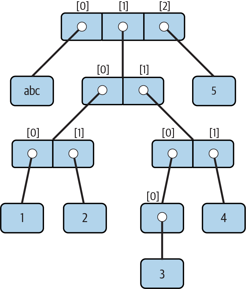
Figure 9-1. A nested object tree with the offsets of its components
References Versus Copies
Chapter 6 mentioned that assignments always store references to objects, not copies of those objects. In practice, this is usually what you want. Because assignments can generate multiple references to the same object, though, it’s important to be aware that changing a mutable object in place may affect other references to the same object elsewhere in your program. If you don’t want such behavior, you’ll need to tell Python to copy the object explicitly.
We studied this phenomenon in Chapter 6, but it can become more subtle when larger objects of the sort we’ve explored since then come into play. For instance, the following example creates a list assigned to X, and another list assigned to L that embeds a reference back to list X. It also creates a dictionary D that contains another reference back to list X:
>>>X = [1, 2, 3]>>>L = ['a', X, 'b']# Embed references to X's object in two others>>>D = {'x':X, 'y':2}
At this point, there are three references to the first list created: from the name X, from inside the list assigned to L, and from inside the dictionary assigned to D. The situation is illustrated in Figure 9-2.
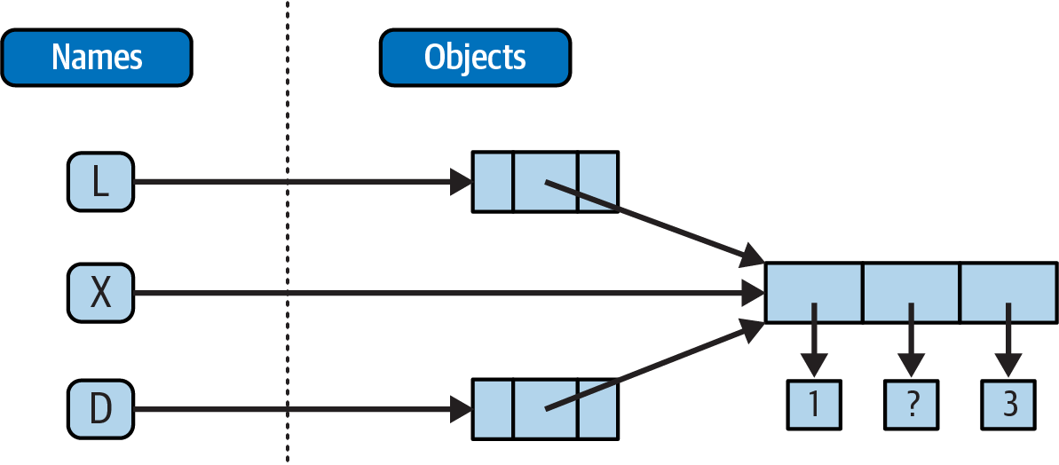
Figure 9-2. Shared objects: changing from X makes it look different from L and D too
Because lists are mutable, changing the shared list object from any of the three references also changes what the other two reference:
>>>X[1] = 'surprise'# Changes all three references!>>>L['a', [1, 'surprise', 3], 'b'] >>>D{'x': [1, 'surprise', 3], 'y': 2}
References are a higher-level analogue of pointers in other languages that are always followed when used. Although you can’t grab hold of the reference itself, it’s possible to store the same reference in more than one place (variables, lists, and so on). This is a feature—you can pass a large object around a program without generating expensive copies of it along the way. If you really want to avoid the potential side effects of shared references, however, you can request copies, in one of a number of ways:
Slice expressions with empty limits (
L[:]) copy sequences.The dictionary, set, and list
copymethod (X.copy()) copies a dictionary, set, or list.Some built-in functions, such as
listanddictmake copies (list(L),dict(D),set(S)).The
copystandard library module makes full (“recursive”) copies when needed.
For example, say you have a list and a dictionary, and you don’t want their values to be changed through other variables:
>>>L = [1,2,3]>>>D = {'a':1, 'b':2}
To prevent this, simply assign copies to the other variables, not references to the same objects:
>>>A = L[:]# Instead of A = L (or list(L), L.copy())>>>B = D.copy()# Instead of B = D (ditto for sets)
This way, changes made from the other variables will change the copies, not the originals:
>>>A[1] = 'Py'>>>B['c'] = 'code'# Changes copies, not originals>>> >>>L, D([1, 2, 3], {'a': 1, 'b': 2}) >>>A, B([1, 'Py', 3], {'a': 1, 'b': 2, 'c': 'code'})
In terms of our original example, you can avoid the reference side effects by slicing the original list instead of simply naming it:
>>>X = [1, 2, 3]>>>L = ['a', X[:], 'b']# Embed copies of X's object>>>D = {'x':X[:], 'y':2}
This changes the picture in Figure 9-2—L and D will now point to different lists than X. The net effect is that changes made through X will impact only X, not L and D; similarly, changes to L or D will not impact X.
One final note on copies: empty-limit slices and the dictionary copy method only make top-level copies; that is, they do not copy nested data structures, if any are present. If you need a complete, fully independent copy of a deeply nested data structure (like the various record structures we’ve coded in recent chapters), use the standard copy module, introduced in Chapter 6:
import copyX= copy.deepcopy(Y)# Fully copy an arbitrarily nested object Y
This call traverses objects to copy all their parts, no matter how deep they may be. This is a much rarer case, though, which is why you have to say more to use this scheme. References are usually what you will want; when they are not, slices and copy methods are usually as much copying as you’ll need to do.
Comparisons, Equality, and Truth
All Python objects also respond to comparisons: tests for equality, relative magnitude, and so on. We’ve seen comparison at work on specific objects in earlier chapters but can finally summarize the general rules.
In short, Python comparisons always inspect all parts of compound objects until a result can be determined. When nested objects are present, Python automatically traverses data structures to apply comparisons from left to right, and as deeply as needed. The first difference found along the way determines the comparison result.
This is sometimes called a recursive comparison—the same comparison requested on the top-level objects is applied to each of the nested objects, and to each of their nested objects, and so on, until a result is found. Later in this book (Chapter 19) you’ll learn how to write recursive functions of your own that work similarly on nested structures. For now, think about comparing all the linked pages at two websites if you want a metaphor for such structures, and a reason for writing recursive functions to process them.
In terms of core objects, the recursion is automatic. For instance, a comparison of list objects compares all their components automatically until a mismatch is found or the end is reached:
>>>L1 = [1, ('a', 3)]# Same value, but different objects>>>L2 = [1, ('a', 3)]>>>L1 == L2, L1 is L2# Same value? Same object?(True, False)
Here, L1 and L2 are assigned lists that are equivalent but distinct objects. As a review of Chapter 6’s coverage, because of the nature of Python references, there are two ways to test for equality:
The
==operator tests value equivalence. Python performs an equivalence test, comparing all nested objects recursively.The
isoperator tests object identity. Python tests whether the two are really the same object (i.e., live at the same address in memory).
In the preceding example, L1 and L2 pass the == test (they have equivalent values because all their components are equivalent) but fail the is check (they reference two different objects, and hence two different pieces of memory). Notice what happens for short strings, though:
>>>S1 = 'text'>>>S2 = 'text'>>>S1 == S2, S1 is S2(True, True)
Here, we should again have two distinct objects that happen to have the same value: == should be true, and is should be false. But because Python internally caches and reuses some objects as an optimization, there really is just a single string 'text' in memory, shared by S1 and S2. Hence, the is identity test reports a true result. To trigger the normal behavior, we need to use strings that are longer (or otherwise defeat caching rule prone to change over time):
>>>S1 = 'a longer string'>>>S2 = 'a longer string'>>>S1 == S2, S1 is S2(True, False)
Of course, because strings are immutable, the object caching mechanism is irrelevant to your code—strings can’t be changed in place, regardless of how many variables refer to them. If identity tests seem confusing, see Chapter 6 for a refresher on object reference concepts. As a rule of thumb, the == operator is what you will want to use for almost all equality checks; is is reserved for highly specialized roles. You’ll see use cases for both later.
As demoed along the way, relative magnitude comparisons are also applied recursively to nested data structures:
>>>L1 = [1, ('a', 3)]# Nested 3 > nested 2>>>L2 = [1, ('a', 2)]>>>L1 < L2, L1 == L2, L1 > L2# Less, equal, greater: tuple of results(False, False, True)
Here, L1 is greater than L2 because the nested 3 is greater than the nested 2. More broadly, Python compares its core object types as follows:
Numbers are compared by relative magnitude, after conversion to the common highest type if needed (e.g.,
1 < 1.1after1is replaced with1.0)Strings are compared lexicographically (by the character code-point values returned by
ord), and character by character until the end or first mismatch (e.g.,'abc' < 'ac').Lists and tuples are compared by comparing each component from left to right, and recursively for nested structures, until the end or first mismatch (e.g.,
[1, 3] > [1, 2]).Sets are equal if both contain the same items (formally, if each is a subset of the other), and magnitude comparison operators for sets apply subset and superset tests.
Dictionaries compare as equal if their sorted
(key, value)lists are equal. Magnitude comparisons are not supported for dictionaries but can be coded by comparing manually sorteditemsresults.Nonnumeric mixed-type magnitude comparisons (e.g.,
1 < 'text') are errors. By proxy, this also applies to sorts, which use comparisons internally: nonnumeric mixed-type collections cannot be sorted sans conversions.
In general, comparisons of structured objects proceed as though you had written the objects as literals and compared all their parts one at a time from left to right. In later chapters, you’ll also see that class-based objects can change the way they are compared. Here, the following sections provide a few more details on Python’s built-in comparisons.
Mixed-type comparisons and sorts
The preceding section’s last bullet point applies only to nonnumeric mixed-type magnitude tests, not equality, but it also applies by proxy to sorting, which does magnitude testing internally. Python disallows mixed-type magnitude testing, except for numeric types and manually converted types:
>>>11 == '11'# Equality works but magnitude does notFalse >>>11 >= '11'TypeError: '>=' not supported between instances of 'int' and 'str' >>>['11', '22'].sort()# Ditto for sorts>>>[11, '11'].sort()TypeError: '<' not supported between instances of 'str' and 'int' >>>11 > 9.123# Mixed numbers convert to highest typeTrue >>>str(11) >= '11', 11 >= int('11')# Manual conversions force the issue(True, True)
Dictionary comparisons
As noted in Chapter 8, magnitude comparisons don’t work for dictionaries directly. Though subject to implementation morph, this purportedly reflects that fact that magnitude comparison would incur too much overhead and may hamper the more common equality test, which may use an optimized scheme that doesn’t compare sorted key/value lists:
>>>D1 = {'b':3, 'a':1}>>>D2 = {'a':1, 'b':3}>>>D1 == D2# Equality, not magnitudeFalse >>>D1 < D2TypeError: '<' not supported between instances of 'dict' and 'dict'
To work around this limitation, either write loops to compare values by key, or, as also shown in Chapter 8, simply compare sorted key/value lists manually by combining the items dictionary method and sorted built-in:
>>>list(D1.items())[('b', 3), ('a', 1)] >>>sorted(D1.items())[('a', 1), ('b', 3)] >>>sorted(D1.items()) < sorted(D2.items())# Dictionary magnitude testsFalse >>>sorted(D1.items()) >= sorted(D2.items())True
This takes more code than a simple < or > and may run relatively slowly; but in practice, most programs requiring this behavior either will develop more efficient ways to compare data in dictionaries or won’t care about the sloth.
The Meaning of True and False in Python
Notice that the test results returned in the last two examples represent true and false values. They print as the words True and False, but now that we’re using logical tests like these in earnest, it’s time to be a bit more formal about what these names really mean.
In Python, as in most programming languages, an integer 0 represents false, and an integer 1 represents true (a heritage rooted in the digital nature of computer hardware). In addition, though, Python recognizes any empty data structure as false and any nonempty data structure as true. More generally, the notions of true and false are intrinsic properties of every object in Python—each object is either true or false, as follows:
Numbers are false if zero, and true otherwise
Collection objects are false if empty, and true otherwise
The
Noneplaceholder object is always falseTrue and False are preset to true and false, respectively
Table 9-4 gives examples of true and false values of various objects in Python.
| Object | Value |
|---|---|
'text' |
True |
'' |
False |
[1, 2] |
True |
[] |
False |
{'a': 1} |
True |
{} |
False |
1 |
True |
0.0 |
False |
None |
False |
As one application of this, because objects are true or false themselves, it’s common to see Python programmers code tests like if X:, which, assuming X is a string, is the same as if X != '':. In other words, you can test the object itself to see if it contains anything, instead of comparing it to an empty—and therefore false—object of the same type.
The None object
As shown in the last row in Table 9-4, Python also provides a special object called None, which is always considered to be false. None was introduced briefly in Chapter 4; it is the only value of a special data type in Python and typically serves as an empty placeholder (much like a NULL pointer in C).
For example, recall that for lists you cannot assign to an offset unless that offset already exists—the list does not magically grow if you attempt an out-of-bounds assignment. To preallocate a list such that you can store values in any of its offsets, you can fill it with None objects:
>>>size = 50>>>L = []>>>L[size - 1] = 'NO'IndexError: list assignment index out of range >>>L = [None] * size>>>L[size - 1] = 'OK'>>>L[-10:][None, None, None, None, None, None, None, None, None, 'OK']
This doesn’t limit the size of the list (it can still grow and shrink later), but simply presets an initial size to allow for future index assignments. You could initialize a list with zeros the same way, of course, but best practice suggests using None if the type of the list’s contents is variable or not yet known.
Keep in mind that None does not mean “undefined.” That is, None is something, not nothing (despite its name!)—it is a real object and a real piece of memory that is created and given a built-in name by Python itself. Watch for other uses of this special object later in the book; as you’ll learn in Part IV, it is also the default return value of functions that don’t exit by running into a return statement with a result value.
The bool type
While we’re on the topic of truth, also keep in mind that the Python Boolean type bool, introduced in Chapter 5, simply augments the notions of true and false in Python. As we learned earlier, the built-in words True and False are just customized versions of the integers 1 and 0—it’s as if these two words have been preassigned to 1 and 0 everywhere in Python. Because of the way this new type is implemented, this is really just a minor extension to the notions of true and false already described, designed to make truth values more explicit:
When used explicitly in truth test code, the words
TrueandFalseare equivalent to1and0, respectively, but they make the programmer’s intent clearer.Results of Boolean tests run interactively print as the words
TrueandFalse, instead of as1and0, to make the type of result clearer.
You are not required to use only Boolean types in logical statements such as if; all objects are still inherently true or false, and all the Boolean concepts mentioned in this chapter still work as described if you use other types. Python also provides a bool built-in function that can be used to extract the Boolean value of an object. You can use this to explicitly check if an object is true—that is, nonzero or nonempty:
>>>bool(1)True >>>bool('text')True >>>bool({})False
In practice, though, you’ll rarely notice the Boolean type produced by logic tests, because Boolean results are used automatically by if statements and other selection tools. We’ll explore Booleans further when we study logical statements in Chapter 12.
Python’s Type Hierarchies
As a summary and reference, Figure 9-3 sketches all the major built-in object types available in Python and their relationships. We’ve explored the most prominent of these in this part of the book. Other objects in Figure 9-3 are program units (e.g., functions and modules) or interpreter internals (e.g., stack frames and compiled code).
The main point to notice here is that everything processed in a Python program is an object type. This is sometimes called a “first class” object model, because all objects are on equal footing with respect to your code. For instance, you can pass a class to a function, assign it to a variable, stuff it in a list or dictionary, and so on.
Type Objects
In fact, even types themselves are an object type in Python: the type of an object is an object of type type (and not just because it’s a decent tongue twister!). Seriously, a call to the built-in function type(X) returns the type object of object X. The practical application of this is that type objects can be used for manual type comparisons in Python if statements. However, for reasons introduced in Chapter 4 that we won’t rehash here, manual type testing is usually not the right thing to do in Python, since it limits your code’s flexibility. Python is about flexibility, not constraints.
One note on type names: each core type has a built-in name that supports various roles, including type customization through object-oriented subclassing: dict, list, str, tuple, int, float, complex, bytes, type, set, and more. Technically speaking, these names reference classes, and calls to these names are really object constructor calls, not simply conversion functions, though you can treat them as simple functions for basic usage.
In addition, the types standard library module provides additional type names for types that are not available as built-ins (e.g., types.FunctionType is the is the type of functions), and the isinstance built-in function checks types with consideration of inheritance in OOP—a topic we’ll reach later on our Python journey. Because types can be customized with OOP in Python, though, the isinstance technique is generally recommended in the very rare cases where code must know about specific types. There’s more on type customizations in Chapter 32, and an example in which isinstance is useful and warranted in Chapter 19.
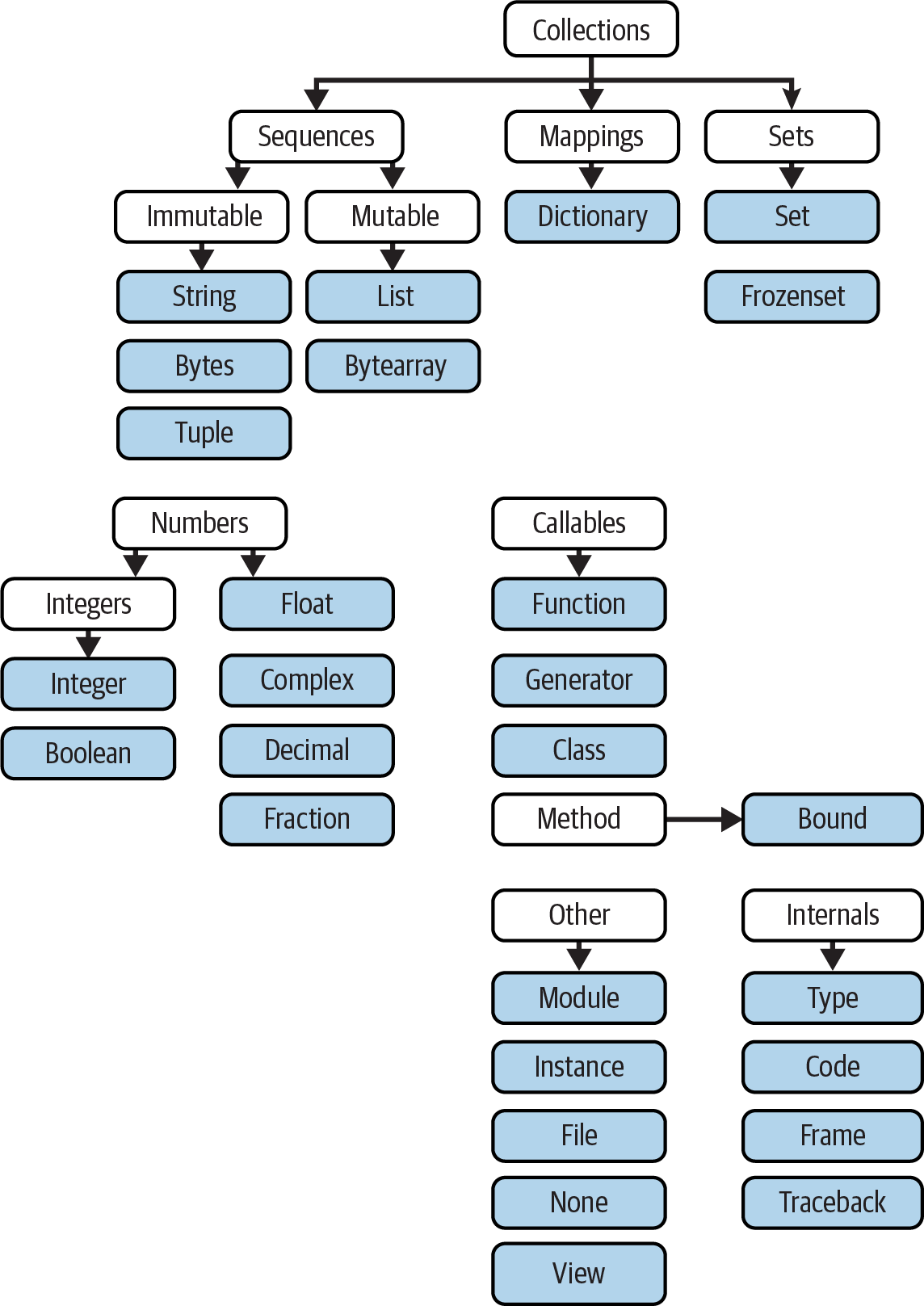
Figure 9-3. Python’s major built-in object types, organized by categories
Other Types in Python
Besides the core objects studied in this part of the book, and the program-unit objects such as functions, modules, and classes that you’ll meet later, a typical Python installation has dozens of additional object types available as linked-in C extensions or imported Python classes—regular expression objects, GUI widgets, network sockets, and so on. Depending on whom you ask, the named tuple you met earlier in this chapter may fall in this category too, along with Decimal and Fraction of Chapter 5.
The main difference between these extra tools and the built-in types you’ve seen so far is that the built-ins have language-defined syntax for creating their objects (e.g., 4 for an integer, [1,2] for a list, the open function for files, and def and lambda for functions). Other tools are made available in standard library modules that you import to use. For instance, to make a regular-expression object in pattern matching, you import re and call re.compile().
Because most objects in this noncore category are application-level tools that are beyond the scope of this language tutorial, be sure to browse Python’s library reference early and often in your coding career for a comprehensive chronicle of all the supplemental tools available to Python programs.
Note
What about range?: Python’s documentation reclassified the built-in range function as a sequence type, along with lists and tuples, but this is an academic sleight of hand that we won’t adhere to in this book. As you’ll see later, range returns an iterable object which produces results on demand, not a physically stored sequence. It supports some—but not all—sequence operations (e.g., indexing works but concatenation does not), but even this is an implementation trick, and hardly enough to constitute a new type on the same level as real sequences. Labeling range an “immutable sequence of integers” conflates tool categories and confuses Python learners.
Built-in Type Gotchas
That’s the end of our look at core data types. We’ll wrap up this part of the book with a discussion of common problems that seem to trap new users (and the occasional expert), along with their solutions. Some of this is a review of ideas we’ve already covered, but these issues are important enough to warrant callouts again here.
Assignment Creates References, Not Copies
Yes, this is redundant, but it’s such a common pitfall that it’s worth underscoring one more time: shared references to mutable objects can matter. In the following, for instance, the list object assigned to the name L is referenced both from L and from inside the list assigned to the name M. Changing L in place changes what M references, too:
>>>L = [1, 2, 3]>>>M = ['X', L, 'Y']# Embed a reference to L>>>M['X', [1, 2, 3], 'Y'] >>>L[1] = 0# Changes M (what M references) too>>>M['X', [1, 0, 3], 'Y']
This effect usually becomes important only in larger programs, and shared references are often exactly what you want. If objects change out from under you in ways unexpected and unwanted, though, you can avoid sharing objects easily by copying them explicitly. For lists, you can always make a top-level copy by using an empty-limits slice, among other techniques described earlier in this chapter:
>>>L = [1, 2, 3]>>>M = ['X', L[:], 'Y']# Embed a copy of L>>>L[1] = 0# Changes only L, not M>>>L[1, 0, 3] >>>M['X', [1, 2, 3], 'Y']
Remember, slice limits default to 0 and the length of the sequence being sliced; if both are omitted, the slice extracts every item in the sequence and so makes a top-level copy (a new, unshared object).
Repetition Adds One Level Deep
As we’ve learned, repeating a sequence is like adding it to itself a number of times. However, when mutable sequences are nested, the effect might not always be what you expect. For instance, in the following example X is assigned to L repeated four times, whereas Y is assigned to a list containing L repeated four times:
>>>L = [4, 5, 6]>>>X = L * 4# Like [4, 5, 6] + [4, 5, 6] + …>>>Y = [L] * 4# [L] + [L] + … = [L, L, …]>>>X[4, 5, 6, 4, 5, 6, 4, 5, 6, 4, 5, 6] >>>Y[[4, 5, 6], [4, 5, 6], [4, 5, 6], [4, 5, 6]]
Subtly, because L was nested in the second repetition, Y winds up embedding references back to the original list assigned to L, and so is open to the same sorts of side effects noted in the preceding section:
>>>L[1] = 0# Impacts Y but not X>>>X[4, 5, 6, 4, 5, 6, 4, 5, 6, 4, 5, 6] >>>Y[[4, 0, 6], [4, 0, 6], [4, 0, 6], [4, 0, 6]]
This may seem artificial and academic—until it happens unexpectedly in your code! The same solutions to this problem apply here as in the previous section, as this is really just another way to create the shared mutable object reference case—make copies when you don’t want shared references:
>>>L = [4, 5, 6]>>>Y = [list(L)] * 4# Embed a (shared) copy of L>>>L[1] = 0>>>Y[[4, 5, 6], [4, 5, 6], [4, 5, 6], [4, 5, 6]]
Even more subtly, although Y doesn’t share an object with L anymore, it still embeds four references to the same copy of it. If you must avoid that sharing too, you’ll want to make sure each embedded copy is unique:
>>>Y[0][1] = 99# All four copies are still the same>>>Y[[4, 99, 6], [4, 99, 6], [4, 99, 6], [4, 99, 6]] >>>L = [4, 5, 6]>>>Y = [list(L) for i in range(4)]>>>Y[[4, 5, 6], [4, 5, 6], [4, 5, 6], [4, 5, 6]] >>>Y[0][1] = 99# And now they're not!>>>Y[[4, 99, 6], [4, 5, 6], [4, 5, 6], [4, 5, 6]]
If you remember that repetition, concatenation, and slicing copy only the top level of their operand objects, these sorts of cases make much more sense.
Beware of Cyclic Data Structures
We encountered this concept in a prior exercise but didn’t explore it much: if a collection object contains a reference to itself, it’s called a cyclic object. Python prints a [...] whenever it detects a cycle in the object back to itself, rather than getting stuck in an infinite loop (as it once did long ago, when dinosaurs roamed the planet):
>>>L = ['stuff']# Append reference to same object>>>L.append(L)# Makes a cycle back to the same object: [...]>>>L['stuff', [...]]
Besides understanding that the three dots in square brackets represent a cycle in the object (should they ever crop up in your outputs or job interviews!), this case is worth knowing about because it can lead to real gotchas—cyclic structures may cause code of your own to fall into unexpected loops if you don’t anticipate them.
For instance, some programs that walk through structured data must keep a list, dictionary, or set of already visited items, and check it when they’re about to step into a cycle that could cause an unwanted loop. See the Part I exercise solutions in “Part I, Getting Started” in Appendix B for more on this problem. Also watch for general discussion of recursion in Chapter 19, as well as the reloadall.py program in Chapter 25 and the ListTree class in Chapter 31 for concrete examples of programs where cycle detection can matter.
As is so often the case in programming, the solution is knowledge: don’t use cyclic references unless you really need to, and make sure you anticipate them in programs that must care. There are good reasons to create cycles, but unless you have code that knows how to handle them, objects that reference themselves may be more liability than asset. They need not, however, also be a surprise.
Immutable Types Can’t Be Changed in Place
And just once more for completeness: you cannot change an immutable object in place. Instead, you construct a new object with slicing, concatenation, and so on, and assign it back to the original reference, if needed:
T = (1, 2, 3) T[2] = 4# Error!T = T[:2] + (4,)# OK: (1, 2, 4)
That might seem like extra coding work (and it is), but the upside is that most of the previous gotchas in this section can’t happen when you’re using immutable objects like tuples and strings; because they can’t be changed in place, they are not generally open to the sorts of side effects that can imperil mutable objects like lists and dictionaries.
Chapter Summary
This chapter explored the last two major core object types—the tuple and the file. We learned that tuples support all the usual sequence operations, have just a few methods, do not allow any in-place changes because they are immutable, and are generalized by the named-tuple extension type. We also learned that files are returned by the built-in open function and provide methods for reading and writing content of both the text and binary kind.
Along the way we explored how to translate Python objects to and from strings for storing in files, and we looked at pickle, json, and other modules for advanced roles (object serialization and binary data). Finally, we wrapped up by reviewing some properties common to all object types (e.g., shared references) and went through a list of common mistakes (“gotchas”) in the object-type domain.
In the next part of this book, we’ll shift gears, turning to the topic of statement syntax—the way we code processing steps and logic in our scripts. Along the way, this next part explores all of Python’s basic procedural statements. The next chapter kicks off this topic with an introduction to Python’s general syntax model, which is applicable to all statement types. Before moving on, though, take the chapter quiz, and then work through the end-of-part lab exercises to review type concepts. The next part’s statements largely just create and process objects, so make sure you’ve mastered this domain by working through all the exercises before reading on.
Test Your Knowledge: Quiz
How can you determine how large a tuple is? Why is this tool located where it is?
Write an expression that changes the first item in a tuple.
(4, 5, 6)should become(1, 5, 6)in the process.What is the default for the processing mode argument in a file
opencall?What module might you use to store Python objects in a file without converting them to strings yourself?
How might you go about copying all parts of a nested structure at once?
When does Python consider an object to be true?
Test Your Knowledge: Answers
The built-in
lenfunction returns the length (number of contained items) for any container object in Python, including tuples. It is a built-in function instead of a type method because it applies to many different types of objects. In general, built-in functions and expressions may span many object types; methods are specific to a single object type, though some method names may be available on more than one type (index, for example, works on lists and tuples).Because they are immutable, you can’t really change tuples in place, but you can generate a new tuple with the desired value. Given
T = (4, 5, 6), you can change the first item by making a new tuple from its parts by slicing and concatenating:T = (1,) + T[1:]. (Recall that single-item tuples require a trailing comma.) You could also convert the tuple to a list, change it in place, and convert it back to a tuple, but this is more expensive and is rarely required in practice—simply use a list if you know that the object will require in-place changes.The default for the processing mode argument in a file
opencall is'r', for reading text input. For input text files, simply pass in the external file’s name or path (unless you also need to customize things like buffering policies or provide a Unicode text encoding to override your platform’s default—as fleshed out in Chapter 37).The
picklemodule can be used to store Python objects in a file without explicitly converting them to strings.jsonsimilarly converts a limited set of Python objects to and from strings per the JSON format. Thestructmodule is related, but it assumes the data is to be in packed binary format in the file.Import the
copymodule, and callcopy.deepcopy(X)if you need to copy all parts of a nested structureX. This is also rarely needed in practice; references are usually the desired behavior, and shallow copies (e.g.,aList[:],aDict.copy(),set(aSet)) usually suffice for most copies.An object is considered true if it is either a nonzero number or a nonempty collection object. The built-in words
TrueandFalseare essentially predefined to have the same meanings as integer1and0, respectively.
Test Your Knowledge: Part II Exercises
This session asks you to get your feet wet with coding built-in object fundamentals. As before, a few new ideas may pop up along the way, so be sure to flip to the answers in “Part II, Objects and Operations” in Appendix B when you’re done (or even when you’re not). If you have limited time, consider starting with exercises 10 and 11 (the most practical of the bunch) and then working from first to last as time allows. This is all fundamental material, though, so try to do as many of these as you can; programming is a hands-on activity, and there is no substitute for practicing what you’ve read to make ideas gel.
The basics. Experiment interactively with the common type operations found in the various operation tables in this part of the book. To get started, bring up the Python interactive interpreter (a REPL of your choosing), type each of the following expressions, and try to explain what’s happening in each case. Note that the semicolon in some of these is being used as a statement separator, to squeeze multiple statements onto a single line: for example,
X=1;Xassigns and then prints a variable (more on statement syntax in the next part of the book). Also remember that a comma between expressions usually builds a tuple, even if there are no enclosing parentheses:X,Y,Zis a three-item tuple, which Python prints back to you in parentheses.2 ** 16 2 / 5, 2 / 5.0 'hack' + 'code' S = 'Python' 'grok ' + S S * 5 S[0], S[:0], S[1:] how = 'fun' 'coding %s is %s!' % (S, how) 'coding {} is {}!'.format(S, how) f'coding {S} is {how}!' ('x',)[0] ('x', 'y')[1] L = [1, 2, 3] + [4, 5, 6] L, L[:], L[:0], L[−2], L[−2:] ([1, 2, 3] + [4, 5, 6])[2:4] [L[2], L[3]] L.reverse(); L L.sort(); L L.index(4) {'a': 1, 'b': 2}['b'] D = {'x': 1, 'y': 2, 'z': 3} D['w'] = 0 D['x'] + D['w'] D[(1, 2, 3)] = 4 list(D.keys()), list(D.values()), (1, 2, 3) in D [[]], ["", [], (), {}, None]Indexing and slicing. At the interactive prompt, define a list named
Lthat contains four strings or numbers (e.g.,L=[0, 1, 2, 3]). Then, experiment with the following boundary cases. You may never see these cases in real programs (especially not in the bizarre ways they may appear here!), but they are intended to make you think about the underlying model, and some may be useful in less artificial forms—slicing out of bounds can help, for example, if a sequence is not as long as you expect:What happens when you try to index out of bounds (e.g.,
L[4])?What about slicing out of bounds (e.g.,
L[-1000:100])?Finally, how does Python handle it if you try to extract a sequence in reverse, with the lower bound greater than the higher bound (e.g.,
L[3:1])? Hint: try assigning to this slice (L[3:1]=['?']), and see where the value is put. Do you think this may be the same phenomenon you saw when slicing out of bounds?
Indexing, slicing, and
del. Define another listLwith four items, and assign an empty list to one of its offsets (e.g.,L[2]=[]). What happens? Then, assign an empty list to a slice (L[2:3]=[]). What happens now? Recall that slice assignment deletes the slice and inserts the new value where it used to be.The
delstatement deletes offsets, keys, attributes, and names. Use it on your list to delete an item (e.g.,del L[0]). What happens if you delete an entire slice (del L[1:])? What happens when you assign a nonsequence to a slice (L[1:2]=1)?Tuple assignment. Type the following lines:
>>>
X = 'code'>>>Y = 'hack'>>>X, Y = Y, XWhat do you think is happening to
XandYwhen you type this sequence?Dictionary keys. Consider the following code fragments:
>>>
D = {}>>>D[1] = 'a'>>>D[2] = 'b'You’ve learned that dictionaries aren’t accessed by offsets, so what’s going on here? Does the following shed any light on the subject? (Hint: strings, integers, and tuples share which type category?)
>>>
D[(1, 2, 3)] = 'c'>>>D{1: 'a', 2: 'b', (1, 2, 3): 'c'}Dictionary indexing. Create a dictionary named
Dwith three entries, for keys'a','b', and'c'. What happens if you try to index a nonexistent key (D['d'])? What does Python do if you try to assign to a nonexistent key'd'(e.g.,D['d']='hack')? How does this compare to out-of-bounds assignments and references for lists? Does this sound like the rule for variable names?Generic operations. Run interactive tests to answer the following questions:
What happens when you try to use the
+operator on different/mixed types (e.g., string+list, list+tuple)?Does
+work when one of the operands is a dictionary?Does the
appendmethod work for both lists and strings? How about using thekeysmethod on lists? (Hint: what doesappendassume about its subject object?)Finally, what type of object do you get back when you slice or concatenate two lists or two strings?
String indexing. Define a string
Sof four characters:S = 'hack'. Then type the following expression:S[0][0][0][0][0]. Any clue as to what’s happening this time? (Hint: recall that a string is a collection of characters, but Python characters are one-character strings.) Does this indexing expression still work if you apply it to a list such as['h', 'a', 'c', 'k']? Why?Immutable types. Define a string
Sof four characters again:S = 'hack'. Write an assignment that changes the string to'heck', using only slicing and concatenation. Could you perform the same operation using just indexing and concatenation? How about index assignment?Nesting. Write a data structure that represents your personal information: name (first, middle, last), age, job, address, email address, and phone number. You may build the data structure with any combination of built-in object types you like (lists, tuples, dictionaries, strings, numbers). Then, access the individual components of your data structures by indexing. Do some structures make more sense than others for this object?
Files. Write a script that creates a new output file called myfile.txt and writes the string
'Hello file world!'into it. Then write another script that opens myfile.txt and reads and prints its contents. Run your two scripts from the system command line (or other script-launcher tool available to you). Does the new file show up in the directory where you ran your scripts? What if you add a different directory path to the filename passed toopen? Note: filewritemethods do not add newline characters to your strings; add an explicit\nat the end of the string if you want to fully terminate the line in the file.