14 Duplication
Now it’s time to change gears and dive into another tool you have at your disposal to design horizontally scalable applications — duplication.
14.1 Network load balancing
Arguably the easiest way to add more capacity to a service is to create more instances of it and have some way of routing, or balancing, requests to them. The thinking is that if one instance has a certain capacity, then 2 instances should have a capacity that is twice that.
Creating more service instances can be a fast and cheap way to scale out a stateless service, as long as you have taken into account the impact on its dependencies. For example, if every service instance needs to access a shared data store, eventually, the data store will become a bottleneck, and adding more service instances to the system will only strain it further.
The routing, or balancing, of requests across a pool of servers is implemented by a network load balancer. A load balancer (LB) has one or more physical network interface cards (NIC) mapped to one or more virtual IP (VIP) addresses. A VIP, in turn, is associated with a pool of servers. The LB acts as a middle-man between clients and servers — the clients only see the VIP exposed by the LB and have no visibility of the individual servers associated with it.
Distributing requests across servers has many benefits. Because clients are decoupled from servers and don’t need to know their individual addresses, the number of servers behind the LB can be increased or reduced transparently. And since multiple redundant servers can interchangeably be used to handle requests, a LB can detect faulty ones and take them out of the pool, increasing the service’s availability.
At a high level, a LB supports several core features beyond load balancing, like service discovery and health-checks.
Load Balancing
The algorithms used for routing requests can vary from simple round-robin to more complex ones that take into account the servers’ load and health. There are several ways for a LB to infer the load of the servers. For example, the LB could periodically hit a dedicated load endpoint of each server that returns a measure of how busy the server is (e.g., CPU usage). Hitting the servers constantly can be very costly though, so typically a LB caches these measures for some time.
Using cached, and hence delayed, metrics to distribute requests to servers can create a herding effect. Suppose the load metrics are refreshed periodically, and a server that just joined the pool reported a load of 0 — guess what happens next? The LB is going to hammer that server until the next time its load is sampled. When that happens, the server is marked as busy, and the LB stops sending more requests to it, assuming it hasn’t become unavailable first due to the volume of requests sent its way. This creates a ping-pong effect where the server alternates between being very busy and not busy at all.
Because of this herding effect, it turns out that randomly distributing requests to servers without accounting for their load actually achieves a better load distribution. Does that mean that load balancing using delayed load metrics is not possible?
Actually, there is a way, but it requires combining load metrics with the power of randomness. The idea is to randomly pick two servers from the pool and route the request to the least-loaded one of the two. This approach works remarkably well as it combines delayed load information with the protection against herding that randomness provides.
Service Discovery
Service discovery is the mechanism used by the LB to discover the available servers in the pool it can route requests to. There are various ways to implement it. For example, a simple approach is to use a static configuration file that lists the IP addresses of all the servers. However, this is quite painful to manage and keep up-to-date. A more flexible solution can be implemented with DNS. Finally, using a data store provides the maximum flexibility at the cost of increasing the system’s complexity.
One of the benefits of using a dynamic service discovery mechanism is that servers can be added and removed from the LB’s pool at any time. This is a crucial functionality that cloud providers leverage to implement autoscaling, i.e., the ability to automatically spin up and tear down servers based on their load.
Health checks
Health checks are used by the LB to detect when a server can no longer serve requests and needs to be temporarily removed from the pool. There are fundamentally two categories of health checks: passive and active.
A passive health check is performed by the LB as it routes incoming requests to the servers downstream. If a server isn’t reachable, the request times out, or the server returns a non-retriable status code (e.g., 503), the LB can decide to take that server out from the pool.
Instead, an active health check requires support from the downstream servers, which need to expose a health endpoint signaling the server’s health state. Later in the book, we will describe in greater detail how to implement such a health endpoint.
14.1.1 DNS load balancing
Now that we know what a load balancer’s job is, let’s take a closer look at how it can be implemented. While you probably won’t have to build your own LB given the plethora of off-the-shelf solutions available, a basic knowledge of how load balancing works is crucial. LB failures are very visible to your services’ clients since they tend to manifest themselves as timeouts and connection resets. Because the LB sits between your service and its clients, it also contributes to the end-to-end latency of request-response transactions.
The most basic form of load balancing can be implemented with DNS. Suppose you have a couple of servers that you would like to load balance requests over. If these servers have publicly-reachable IP addresses, you can add those to the service’s DNS record and have the clients pick one when resolving the DNS address, as shown in Figure 14.1.
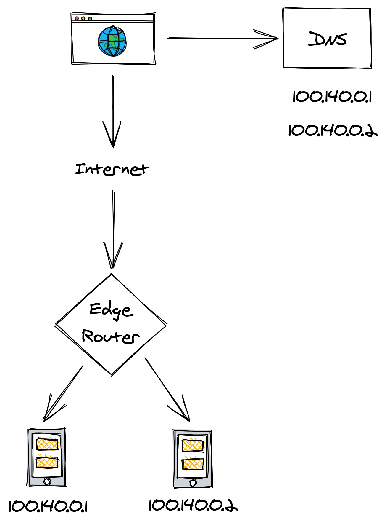
Figure 14.1: DNS load balancing
Although this works, it doesn’t deal well with failures. If one of the two servers goes down, the DNS server will happily continue serving its IP address unaware of the failure. You can manually reconfigure the DNS record to take out the problematic IP, but as we have learned in chapter 4, changes are not applied immediately due to the nature of DNS caching.
14.1.2 Transport layer load balancing
A more flexible load balancing solution can be implemented with a load balancer that operates at the TCP level of the network stack1, through which all traffic between clients and servers needs to go through.
When a client creates a new TCP connection with a LB’s VIP, the LB picks a server from the pool and henceforth shuffles the packets back and forth for that connection between the client and the server. How does the LB assign connections to the servers, though?
A connection is identified by a tuple (source IP/port, destination IP/port). Typically, some form of hashing is used to assign a connection tuple to a server. To minimize the disruption caused by a server being added or removed from the pool, consistent hashing is preferred over modular hashing.
To forward packets downstream, the LB translates each packet’s source address to the LB address and its destination address to the server’s address. Similarly, when the LB receives a packet from the server, it translates its source address to the LB address and its destination address to the client’s address (see Figure 14.2).
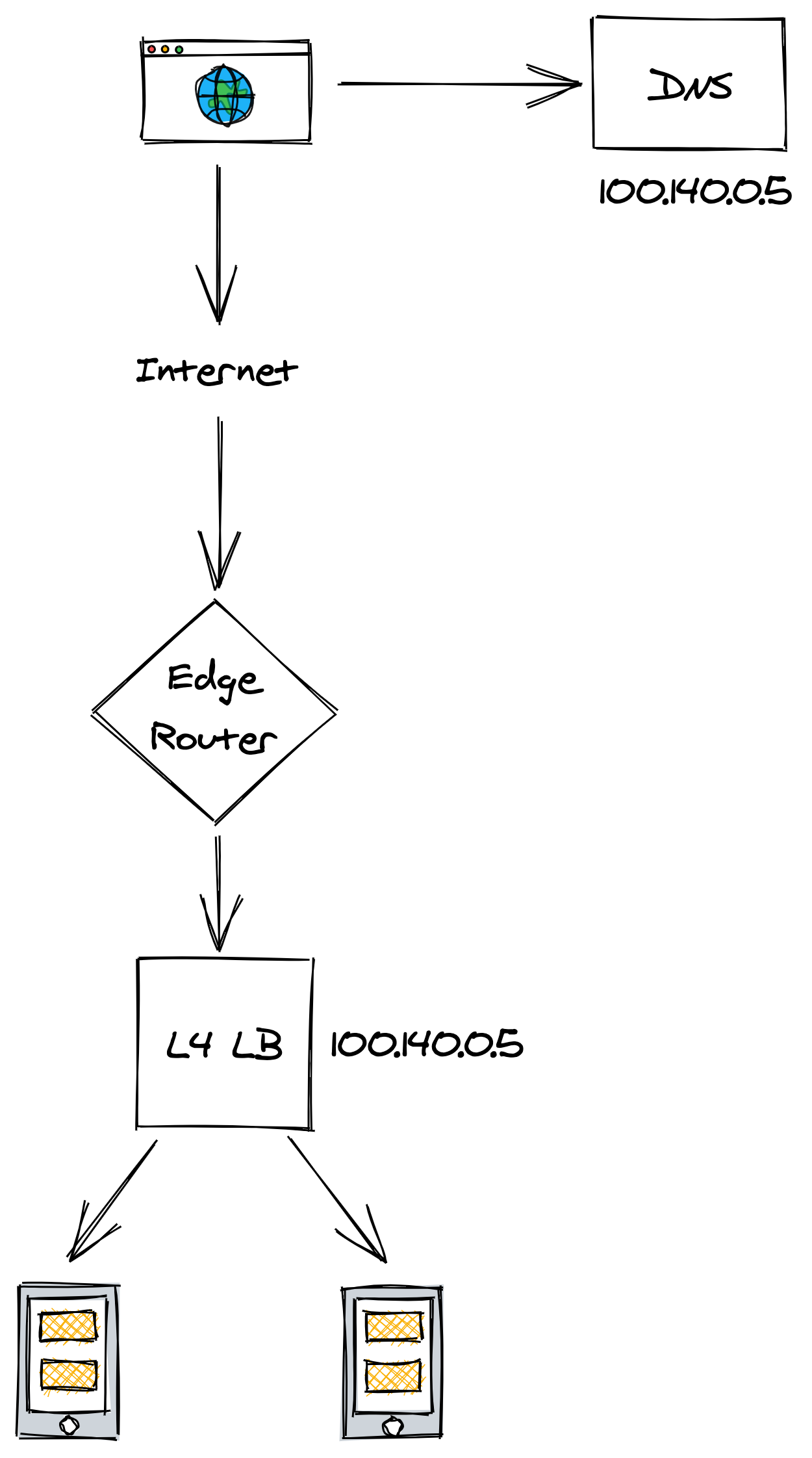
Figure 14.2: Transport layer load balancing
As the data going out of the servers usually has a greater volume than the data coming in, there is a way for servers to bypass the LB and respond directly to the clients using a mechanism called direct server return, but this is beyond the scope of this section.
Because the LB is communicating directly with the servers, it can detect unavailable ones (e.g., with a passive health check) and automatically take them out of the pool improving the reliability of the backend service.
Although load balancing connections at the TCP level is very fast, the drawback is that the LB is just shuffling bytes around without knowing what they actually mean. Therefore, L4 LBs generally don’t support features that require higher-level network protocols, like terminating TLS connections or balancing HTTP sessions based on cookies. A load balancer that operates at a higher level of the network stack is required to support these advanced use cases.
14.1.3 Application layer load balancing
An application layer load balancer2 is an HTTP reverse proxy that farms out requests over a pool of servers. The LB receives an HTTP request from a client, inspects it, and sends it to a backend server.
There are two different TCP connections at play here, one between the client and the L7 LB and another between the L7 LB and the server. Because a L7 LB operates at the HTTP level, it can de-multiplex individual HTTP requests sharing the same TCP connection. This is even more important with HTTP 2, where multiple concurrent streams are multiplexed on the same TCP connection, and some connections can be several orders of magnitude more expensive to handle than others.
The LB can do smart things with application traffic, like rate-limiting requests based on HTTP headers, terminate TLS connections, or force HTTP requests belonging to the same logical session to be routed to the same backend server.
For example, the LB could use a specific cookie to identify which logical session a specific request belongs to. Just like with a L4 LB, the session identifier can be mapped to a server using consistent hashing. The caveat is that sticky sessions can create hotspots as some sessions are more expensive to handle than others.
If it sounds like a L7 LB has some overlapping functionality with an API gateway, it’s because they both are HTTP proxies, and therefore their responsibilities can be blurred.
A L7 LB is typically used as the backend of a L4 LB to load balance requests sent by external clients from the internet (see Figure 14.3). Although L7 LBs offer more functionality than L4 LBs, they have a lower throughput in comparison, which makes L4 LBs better suited to protect against certain DDoS attacks, like SYN floods.
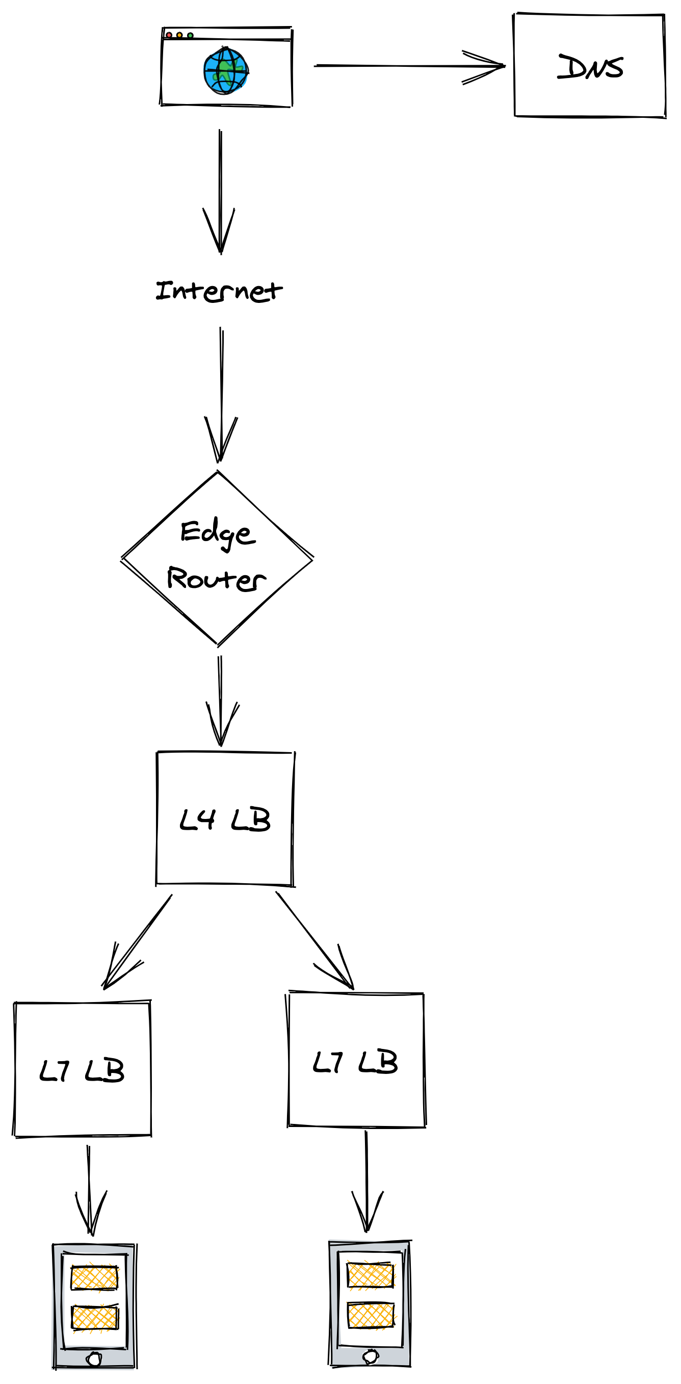
Figure 14.3: A L7 LB is typically used as the backend of a L4 one to load balance requests sent by external clients from the internet.
A drawback of using a dedicated load-balancing service is that all the traffic needs to go through it and if the LB goes down, the service behind it is no longer reachable. Additionally, it’s one more service that needs to be operated and scaled out.
When the clients are internal to an organization, the L7 LB functionality can alternatively be bolted onto the clients directly using the sidecar pattern. In this pattern, all network traffic from a client goes through a process co-located on the same machine. This process implements load balancing, rate-limiting, authentication, monitoring, and other goodies.
The sidecar processes form the data plane of a service mesh, which is configured by a corresponding control plane. This approach has been gaining popularity with the rise of microservices in organizations that have hundreds of services communicating with each other. Popular sidecar proxy load balancers as of this writing are NGINX, HAProxy, and Envoy. The advantage of using this approach is that it distributes the load-balancing functionality to the clients, removing the need for a dedicated service that needs to be scaled out and maintained. The con is a significant increase in the system’s complexity.
14.1.4 Geo load balancing
When we first discussed TCP in chapter 2, we talked about the importance of minimizing the latency between a client and a server. No matter how fast the server is, if the client is located on the other side of the world from it, the response time is going to be over 100 ms just because of the network latency, which is physically limited by the speed of light. Not to mention the increased error rate when sending data across the public internet over long distances.
To mitigate these performance issues, you can distribute the traffic to different data centers located in different regions. But how do you ensure that the clients communicate with the geographically closest L4 load balancer?
This is where DNS geo load balancing comes in — it’s an extension to DNS that considers the location of the client inferred from its IP, and returns a list of the geographically closest L4 LB VIPs (see Figure 14.4). The LB also needs to take into account the capacity of each data center and its health status.
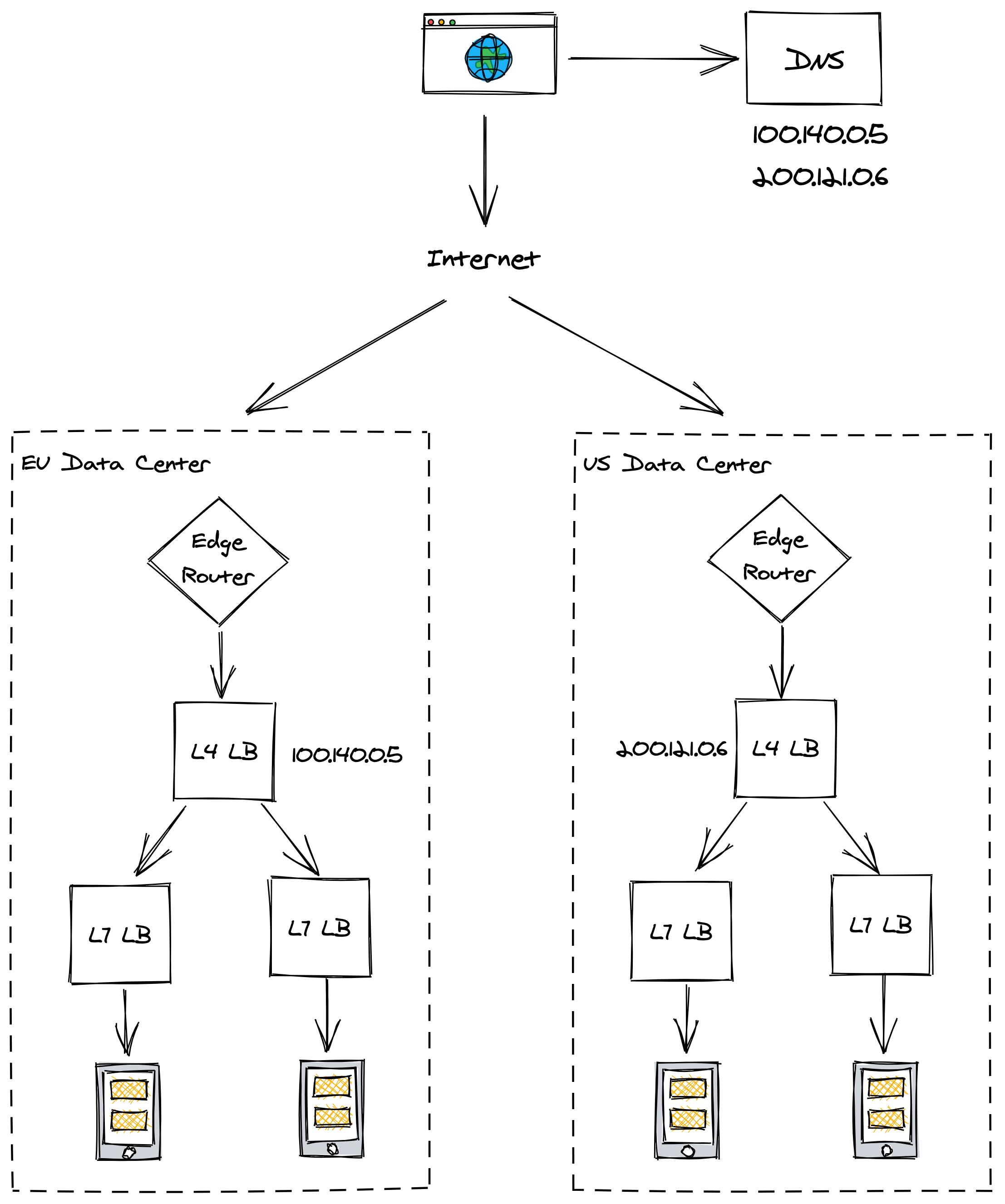
Figure 14.4: Geo load balancing infers the location of the client from its IP
14.2 Replication
If the servers behind a load balancer are stateless, scaling out is as simple as adding more servers. But when there is state involved, some form of coordination is required.
Replication is the process of storing a copy of the same data in multiple nodes. If the data is static, replication is easy: just copy the data to multiple nodes, add a load balancer in front of it, and you are done. The challenge is dealing with dynamically changing data, which requires coordination to keep it in sync.
Replication and sharding are techniques that are often combined, but are orthogonal to each other. For example, a distributed data store can divide its data into N partitions and distribute them over K nodes. Then, a state-machine replication algorithm like Raft can be used to replicate each partition R times (see Figure 14.5).
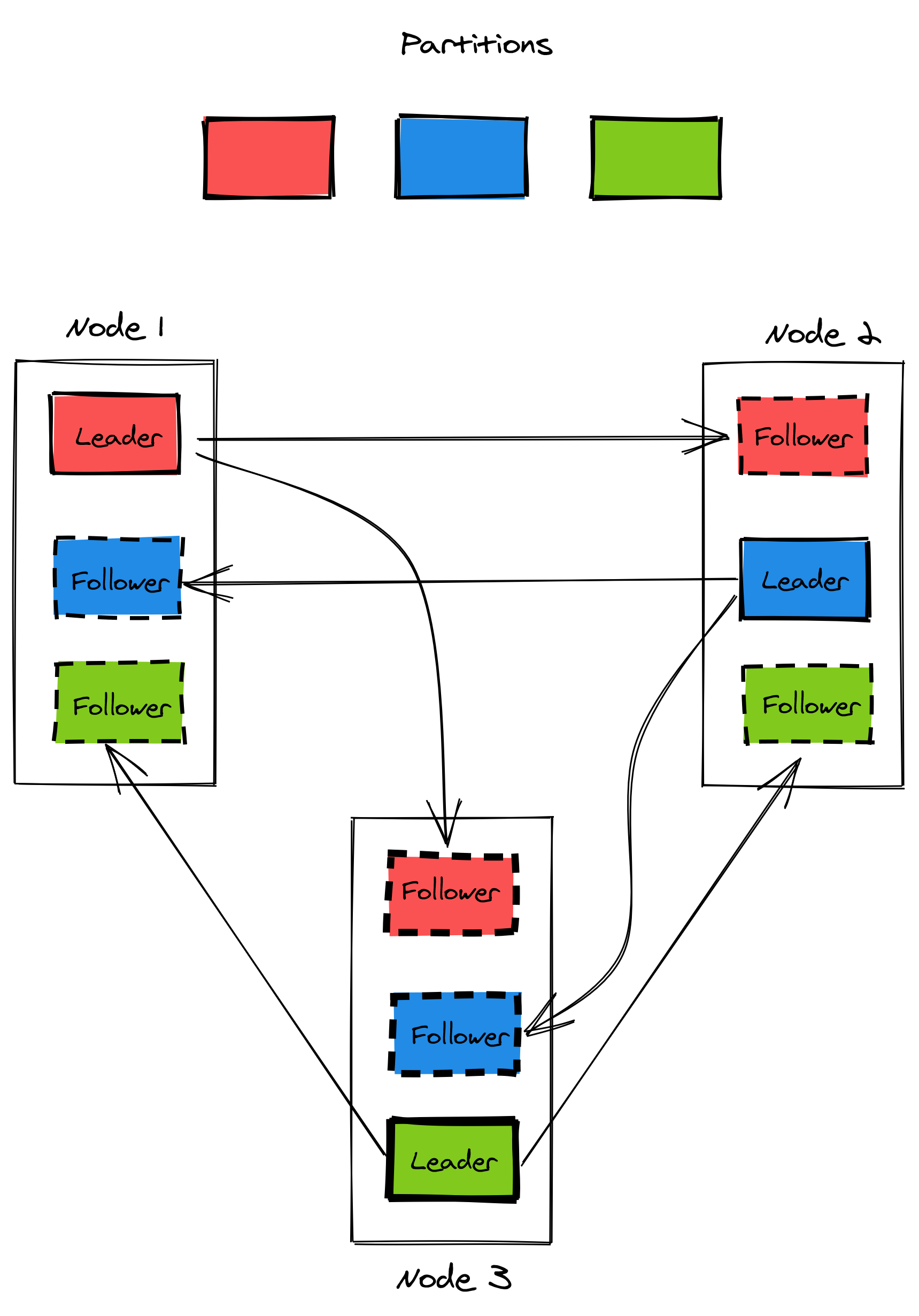
Figure 14.5: A replicated and partitioned data store. A node can be the replication leader for a partition while being a follower for another one.
We have already discussed one way of replicating data in chapter 10. This section will take a broader, but less detailed, look at replication and explore different approaches with varying trade-offs. To keep things simple, we will assume that the dataset is small enough to fit on a single node, and therefore no partitioning is needed.
14.2.1 Single leader replication
The most common approach to replicate data is the single leader, multiple followers/replicas approach (see Figure 14.6). In this approach, the clients send writes exclusively to the leader, which updates its local state and replicates the change to the followers. We have seen an implementation of this when we discussed the Raft replication algorithm.
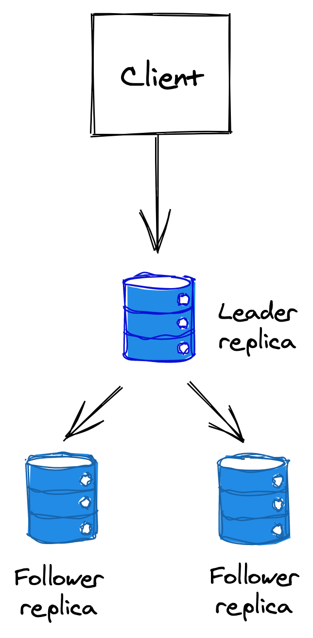
Figure 14.6: Single leader replication
At a high level, the replication can happen either fully synchronously, fully asynchronously, or as a combination of the two.
Asynchronous replication
In this mode, when the leader receives a write request from a client, it asynchronously sends out requests to the followers to replicate it and replies to the client before the replication has been completed.
Although this approach is fast, it’s not fault-tolerant. What happens if the leader crashes right after accepting a write, but before replicating it to the followers? In this case, a new leader could be elected that doesn’t have the latest updates, leading to data loss, which is one of the worst possible trade-offs you can make.
The other issue is consistency. A successful write might not be visible by some or all replicas because the replication happens asynchronously. The client could send a write to the leader and later fail to read the data from a replica because it doesn’t exist there yet. The only guarantee is that if the writes stop, eventually, all replicas will catch up and be identical (eventual consistency).
Synchronous replication
Synchronous replication waits for a write to be replicated to all followers before returning a response to the client, which comes with a performance penalty. If a replica is extremely slow, every request will be affected by it. To the extreme, if any replica is down or not reachable, the store becomes unavailable and it can no longer write any data. The more nodes the data store has, the more likely a fault becomes.
As you can see, fully synchronous or asynchronous replication are extremes that provide some advantages at the expense of others. Most data stores have replication strategies that use a combination of the two. For example, in Raft, the leader replicates its writes to a majority before returning a response to the client. And in PostgreSQL, you can configure a subset of replicas to receive updates synchronously rather than asynchronously.
14.2.2 Multi-leader replication
In multi-leader replication, there is more than one node that can accept writes. This approach is used when the write throughput is too high for a single node to handle, or when a leader needs to be available in multiple data centers to be geographically closer to its clients.
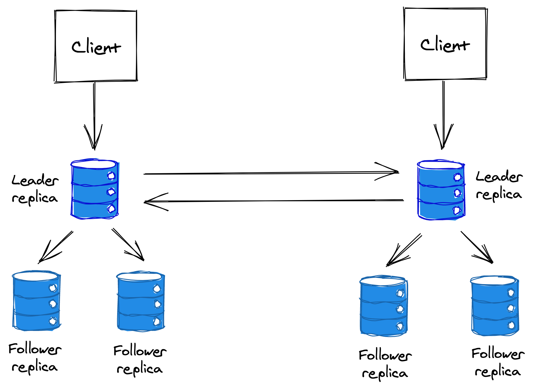
Figure 14.7: Multi-leader replication
The replication happens asynchronously since the alternative would defeat the purpose of using multiple leaders in the first place. This form of replication is generally best avoided when possible as it introduces a lot of complexity. The main issue with multiple leaders are conflicting writes; if the same data item is updated concurrently by two leaders, which one should win? To resolve conflicts, the data store needs to implement a conflict resolution strategy.
The simplest strategy is to design the system so that conflicts are not possible; this can be achieved under some circumstances if the data has a homing region. For example, if all the European customer requests are always routed to the European data center, which has a single leader, there won’t be any conflicting writes. There is still the possibility of a data center going down, but that can be mitigated with a backup data center in the same region, replicated with single-leader replication.
If assigning requests to specific leaders is not possible, and every client needs to be able to write to every leader, conflicting writes will inevitably happen.
One way to deal with a conflict updating a record is to store the concurrent writes and return them to the next client that reads the record. The client will try to resolve the conflict and update the data store with the resolution. In other words, the data store “pushes the can down the road” to the clients.
Alternatively, an automatic conflict resolution method needs to be implemented, for example:
- The data store could use the timestamps of the writes and let the most recent one win. This is generally not reliable because the nodes’ physical clocks aren’t perfectly synchronized. Logical clocks are better suited for the job in this case.
- The data store could allow the client to upload a custom conflict resolution procedure, which can be executed by the data store whenever a conflict is detected.
- Finally, the data store could leverage data structures that provide automatic conflict resolution, like a conflict-free replicated data type (CRDT). CRDTs are data structures that can be replicated across multiple nodes, allowing each replica to update its local version independently from others while resolving inconsistencies in a mathematically sound way.
14.2.3 Leaderless replication
What if any replica could accept writes from clients? In that case, there wouldn’t be any leader(s), and the responsibility of replicating and resolving conflicts would be offloaded entirely to the clients.
For this to work, a basic invariant needs to be satisfied. Suppose the data store has N replicas. When a client sends a write request to the replicas, it waits for at least W replicas to acknowledge it before moving on. And when it reads an entry, it does so by querying R replicas and taking the most recent one from the response set. Now, as long as , the write and replica set intersect, which guarantees that at least one record in the read set will reflect the latest write.
The writes are always sent to all N replicas in parallel; the W parameter determines just the number of responses the client has to receive to complete the request. The data store’s read and write throughput depend on how large or small R and W are. For example, a workload with many reads benefits from a smaller R, but in turn, that makes writes slower and less available.
Like in multi-leader replication, a conflict resolution strategy needs to be used when two or more writes to the same record happen concurrently.
Leaderless replication is even more complex than multi-leader replication, as it’s offloading the leader responsibilities to the clients, and there are edge cases that affect consistency even when is satisfied. For example, if a write succeeded on less than W replicas and failed on the others, the replicas are left in an inconsistent state.
14.3 Caching
Let’s take a look now at a very specific type of replication that only offers best effort guarantees: caching.
Suppose a service requires retrieving data from a remote dependency, like a data store, to handle its requests. As the service scales out, the dependency needs to do the same to keep up with the ever-increasing load. A cache can be introduced to reduce the load on the dependency and improve the performance of accessing the data.
A cache is a high-speed storage layer that temporarily buffers responses from downstream dependencies so that future requests can be served directly from it — it’s a form of best effort replication. For a cache to be cost-effective, there should be a high probability that requested data can be found in it. This requires the data access pattern to have a high locality of reference, like a high likelihood of accessing the same data again and again over time.
14.3.1 Policies
When a cache miss occurs3, the missing data item has to be requested from the remote dependency, and the cache has to be updated with it. This can happen in two ways:
- The client, after getting an “item-not-found” error from the cache, requests the data item from the dependency and updates the cache. In this case, the cache is said to be a side cache.
- Alternatively, if the cache is inline, the cache communicates directly with the dependency and requests the missing data item. In this case, the client only ever accesses the cache.
Because a cache has a maximum capacity for holding entries, an entry needs to be evicted to make room for a new one when its capacity is reached. Which entry to remove depends on the eviction policy used by the cache and the client’s access pattern. One commonly used policy is to evict the least recently used (LRU) entry.
A cache also has an expiration policy that dictates for how long to store an entry. For example, a simple expiration policy defines the maximum time to live (TTL) in seconds. When a data item has been in the cache for longer than its TTL, it expires and can safely be evicted.
The expiration doesn’t need to occur immediately, though, and it can be deferred to the next time the entry is requested. In fact, that might be preferable — if the dependency is temporarily unavailable, and the cache is inline, it can opt to return an entry with an expired TTL to the client rather than an error.
14.3.2 In-process cache
The simplest possible cache you can build is an in-memory dictionary located within the clients, such as a hash-table with a limited size and bounded to the available memory that the node offers.
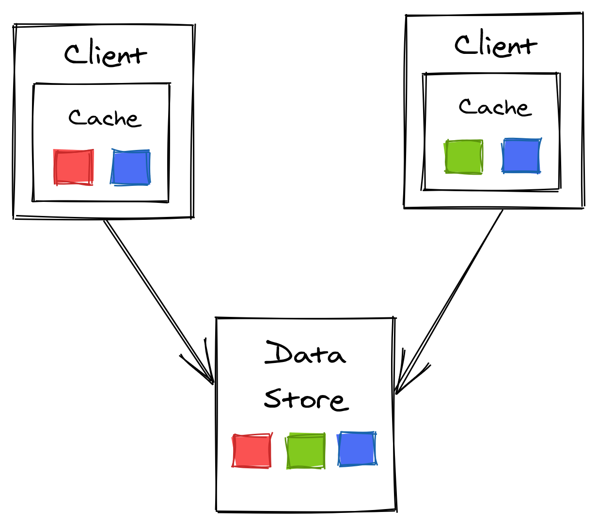
Figure 14.8: In-process cache
Because each cache is completely independent of the others, consistency issues are inevitable since each client potentially sees a different version of the same entry. Additionally, an entry needs to be fetched once per cache, creating downstream pressure proportional to the number of clients.
This issue is exacerbated when a service with an in-process cache is restarted or scales out, and every newly started instance requires to fetch entries directly from the dependency. This can cause a “thundering herd” effect where the downstream dependency is hit with a spike of requests. The same can happen at run-time if a specific data item that wasn’t accessed before becomes all of a sudden very popular.
Request coalescing can be used to reduce the impact of a thundering herd. The idea is that there should be at most one outstanding request at the time to fetch a specific data item per in-process cache. For example, if a service instance is serving 10 concurrent requests requiring a specific record that is not yet in the cache, the instance will send only a single request out to the remote dependency to fetch the missing entry.
14.3.3 Out-of-process cache
An external cache, shared across all service instances, addresses some of the drawbacks of using an in-process cache at the expense of greater complexity and cost.
Because the external cache is shared among the service instances, there can be only a single version of each data item at any given time. And although the cached item can be out-of-date, every client accessing the cache will see the same version, which reduces consistency issues. The load on the dependency is also reduced since the number of times an entry is accessed no longer grows as the number of clients increases.
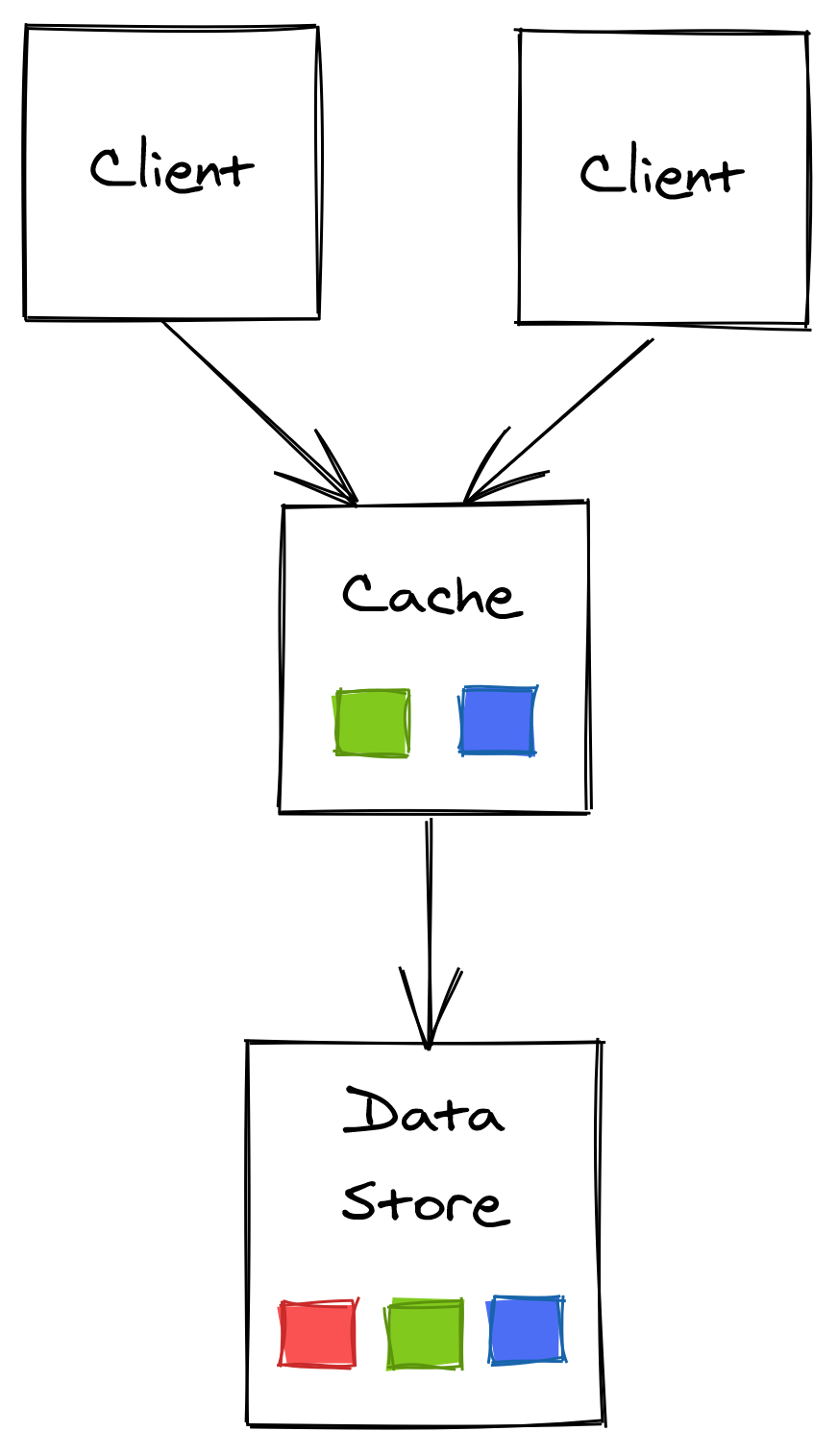
Figure 14.9: Out-of-process cache
Although we have managed to decouple the clients from the dependency, we have merely shifted the load to the external cache. If the load increases, the cache will eventually need to be scaled out. As little data as possible should be moved around when that happens to guarantee that the cache’s availability doesn’t drop and that the number of cache misses doesn’t significantly increase. Consistent hashing, or a similar partitioning technique, can be used to reduce the amount of data that needs to be moved around.
Maintaining an external cache comes with a price as it’s yet another service that needs to be maintained and operated. Additionally, the latency to access it is higher than accessing an in-process cache because a network call is required.
If the external cache is down, how should the service react? You would think it might be okay to temporarily bypass the cache and directly hit the dependency. But in that case, the dependency might not be prepared to withstand a surge of traffic since it’s usually shielded by the cache. Consequently, the external cache becoming unavailable could easily cause a cascading failure resulting in the dependency to become unavailable as well.
The clients can leverage an in-process cache as a defense against the external cache becoming unavailable. Similarly, the dependency also needs to be prepared to handle these sudden “attacks.” Load shedding is a technique that can be used here, which we will discuss later in the book.
What’s important to understand is that a cache introduces a bi-modal behavior in the system4. Most of the time, the cache is working as expected, and everything is fine; when it’s not for whatever reason, the system needs to survive without it. It’s a design smell if your system can’t cope at all without a cache.