13 Partitioning
Now it’s time to change gears and dive into another tool you have at your disposal to scale out application — partitioning or sharding.
When a dataset no longer fits on a single node, it needs to be partitioned across multiple nodes. Partitioning is a general technique that can be used in a variety of circumstances, like sharding TCP connections across backends in a load balancer. To ground the discussion in this chapter, we will anchor it to the implementation of a sharded key-value store.
13.1 Sharding strategies
When a client sends a request to a partitioned data store to read or write a key, the request needs to be routed to the node responsible for the partition the key belongs to. One way to do that is to use a gateway service that can route the request to the right place knowing how keys are mapped to partitions and partitions to nodes.
The mapping between keys and partitions, and other metadata, is typically maintained in a strongly-consistent configuration store, like etcd or Zookeeper. But how are keys mapped to partitions in the first place? At a high level, there are two ways to implement the mapping using either range partitioning or hash partitioning.
13.1.1 Range partitioning
With range partitioning, the data is split into partitions by key range in lexicographical order, and each partition holds a continuous range of keys, as shown in Figure 13.1. The data can be stored in sorted order on disk within each partition, making range scans fast.
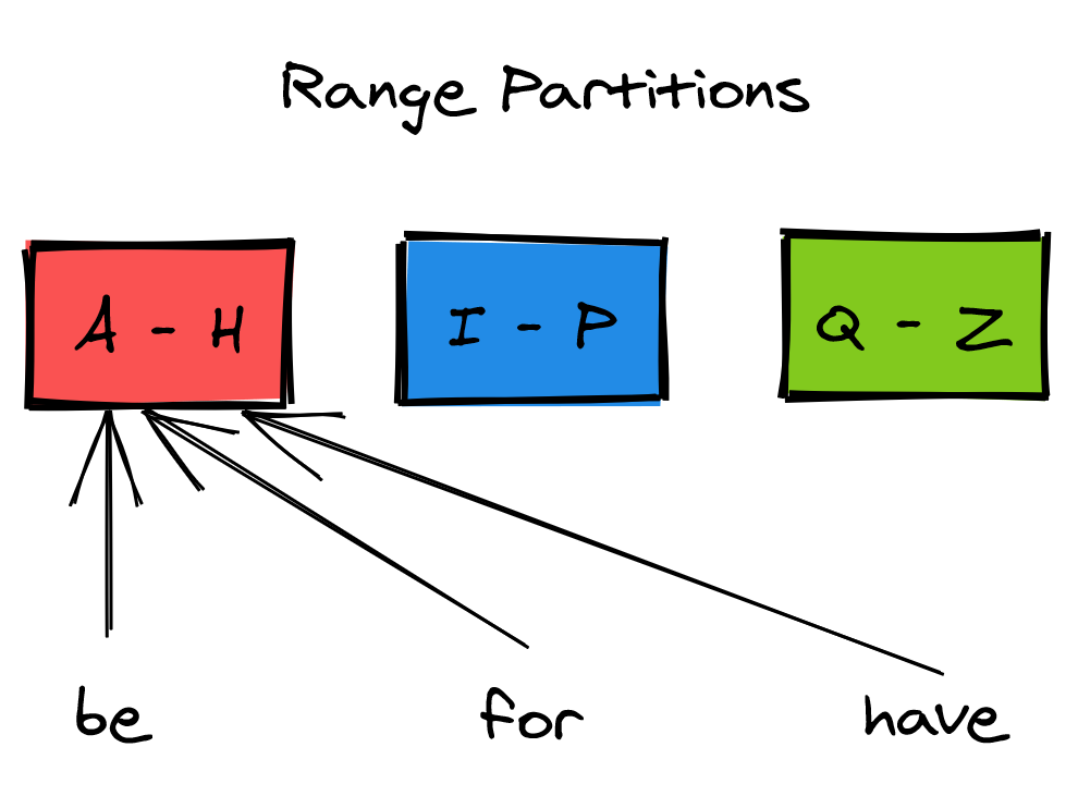
Figure 13.1: A range partitioned dataset
Splitting the key-range evenly doesn’t make much sense though if the distribution of keys is not uniform, like in the English dictionary. Doing so creates unbalanced partitions that contain significantly more entries than others.
Another issue with range partitioning is that some access patterns can lead to hotspots. For example, if a dataset is range partitioned by date, all writes for the current day end up in the same partition, which degrades the data store’s performance.
13.1.2 Hash partitioning
The idea behind hash partitioning is to use a hash function to assign keys to partitions, which shuffles — or uniformly distributes — keys across partitions, as shown in Figure 13.2. Another way to think about it is that the hash function maps a potentially non-uniformly distributed key space to a uniformly distributed hash space.
For example, a simple version of hash partitioning can be implemented with modular hashing, i.e., hash(key) mod N.
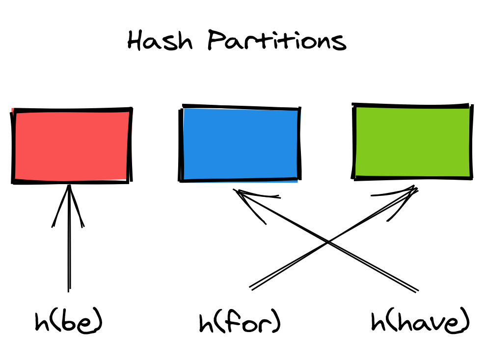
Figure 13.2: A hash partitioned dataset
Although this approach ensures that the partitions contain more or less the same number of entries, it doesn’t eliminate hotspots if the access pattern is not uniform. If there is a single key that is accessed significantly more often than others, then all bets are off. In this case, the partition that contains the hot key needs to be split further down. Alternatively, the key needs to be split into multiple sub-keys, for example, by adding an offset at the end of it.
Using modular hashing can become problematic when a new partition is added, as all keys have to be reshuffled across partitions. Shuffling data is extremely expensive as it consumes network bandwidth and other resources from nodes hosting partitions. Ideally, if a partition is added, only keys should be shuffled around, where is the number of keys and the number of partitions. A hashing strategy that guarantees this property is called stable hashing.
Ring hashing is an example of stable hashing. With ring hashing, a function maps a key to a point on a circle. The circle is then split into partitions that can be evenly or pseudo-randomly spaced, depending on the specific algorithm. When a new partition is added, it can be shown that most keys don’t need to be shuffled around.
For example, with consistent hashing, both the partition identifiers and keys are randomly distributed on a circle, and each key is assigned to the next partition that appears on the circle in clockwise order (see Figure 13.3).
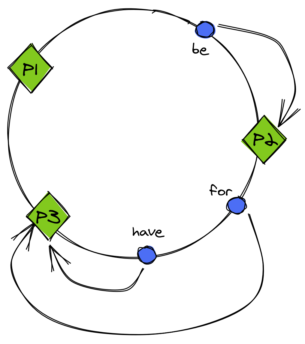
Figure 13.3: With consistent hashing, partition identifiers and keys are randomly distributed on a circle, and each key is assigned to the next partition that appears on the circle in clockwise order.
Now, when a new partition is added, only the keys mapped to it need to be reassigned, as shown in Figure 13.4.
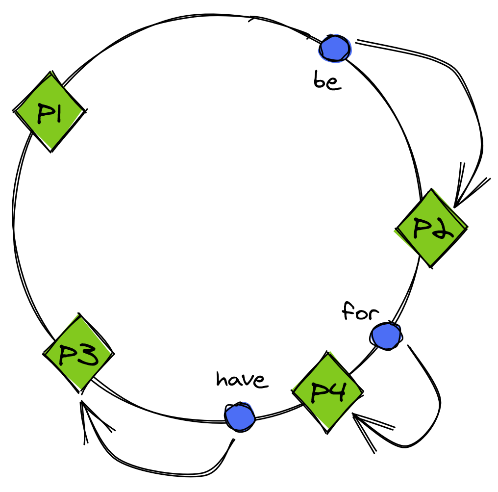
Figure 13.4: After partition P4 is added, key ‘for’ is reassigned to P4, but the other keys are not reassigned.
The main drawback of hash partitioning compared to range partitioning is that the sort order over the partitions is lost. However, the data within an individual partition can still be sorted based on a secondary key.
13.2 Rebalancing
When the number of requests to the data store becomes too large, or the dataset’s size becomes too large, the number of nodes serving partitions needs to be increased. Similarly, if the dataset’s size keeps shrinking, the number of nodes can be decreased to reduce costs. The process of adding and removing nodes to balance the system’s load is called rebalancing.
Rebalancing needs to be implemented in such a way to minimize disruption to the data store, which needs to continue to serve requests. Hence, the amount of data transferred during the rebalancing act needs to be minimized.
13.2.1 Static partitioning
Here, the idea is to create way more partitions than necessary when the data store is first initialized and assign multiple partitions per node. When a new node joins, some partitions move from the existing nodes to the new one so that the store is always in a balanced state.
The drawback of this approach is that the number of partitions is set when the data store is first initialized and can’t be easily changed after that. Getting the number of partitions wrong can be problematic — too many partitions add overhead and decrease the data store’s performance, while too few partitions limit the data store’s scalability.
13.2.2 Dynamic partitioning
An alternative to creating partitions upfront is to create them on-demand. One way to implement dynamic partitioning is to start with a single partition. When it grows above a certain size or becomes too hot, it’s split into two sub-partitions, each containing approximately half of the data. Then, one sub-partition is transferred to a new node. Similarly, if two adjacent partitions become small enough, they can be merged into a single one.
13.2.3 Practical considerations
Introducing partitions in the system adds a fair amount of complexity, even if it appears deceptively simple. Partition imbalance can easily become a headache as a single hot partition can bottleneck the system and limit its ability to scale. And as each partition is independent of the others, transactions are required to update multiple partitions atomically.
We have merely scratched the surface on the topic; if you are interested to learn more about it, I recommend reading Designing Data-Intensive Applications by Martin Kleppmann.