8 Time

8.1 Physical clocks

A process has access to a physical wall-time clock. The most common type is based on a vibrating quartz crystal, which is cheap but not very accurate. The device you are using to read this book is likely using such a clock. It can run slightly faster or slower than others, depending on manufacturing differences and the external temperature. The rate at which a clock runs is also called clock drift. In contrast, the difference between two clocks at a specific point in time is referred to as clock skew.

Because quartz clocks drift, they need to be synced periodically with machines that have access to higher accuracy clocks, like atomic ones. Atomic clocks measure time based on quantum-mechanical properties of atoms and are significantly more expensive than quartz clocks and are accurate to 1 second in 3 million years.

The Network Time Protocol (NTP) is used to synchronize clocks. The challenge is to do so despite the unpredictable latencies introduced by the network. A NTP client estimates the clock skew by correcting the timestamp received by a NTP server with the estimated network latency. Armed with an estimate of the clock skew, the client can adjust its clock, causing it to jump forward or backward in time.

This creates a problem as measuring the elapsed time between two points in time becomes error-prone. For example, an operation that is executed after another could appear to have been executed before.

Luckily, most operating systems offer a different type of clock that is not affected by time jumps: the monotonic clock. A monotonic clock measures the number of seconds elapsed since an arbitrary point, like when the node started up, and can only move forward in time. A monotonic clock is useful to measure how much time elapsed between two timestamps on the same node, but timestamps of different nodes can’t be compared with each other.

Since we don’t have a way to synchronize wall-time clocks across processes perfectly, we can’t depend on them for ordering operations. To solve this problem, we need to look at it from another angle. We know that two operations can’t run concurrently in a single-threaded process as one must happen before the other. This happened-before relationship creates a causal bond between the two operations, as the one that happens first can change the state of the process and affect the operation that comes after it. We can use this intuition to build a different type of clock, one that isn’t tied to the physical concept of time, but captures the causal relationship between operations: a logical clock.

8.2 Logical clocks

A logical clock measures the passing of time in terms of logical operations, not wall-clock time. The simplest possible logical clock is a counter, which is incremented before an operation is executed. Doing so ensures that each operation has a distinct logical timestamp. If two operations execute on the same process, then necessarily one must come before the other, and their logical timestamps will reflect that. But what about operations executed on different processes?

Imagine sending an email to a friend. Any actions you did before sending that email, like drinking coffee, must have happened before the actions your friend took after receiving the email. Similarly, when one process sends a message to another, a so-called synchronization point is created. The operations executed by the sender before the message was sent must have happened before the operations that the receiver executed after receiving it.

A Lamport clock is a logical clock based on this idea. Every process in the system has its own local logical clock implemented with a numerical counter that follows specific rules:

• The counter is initialized with 0.
• The process increments its counter before executing an operation.
• When the process sends a message, it increments its counter and sends a copy of it in the message.
• When the process receives a message, its counter is updated to 1 plus the maximum of its current logical timestamp and the message’s timestamp.

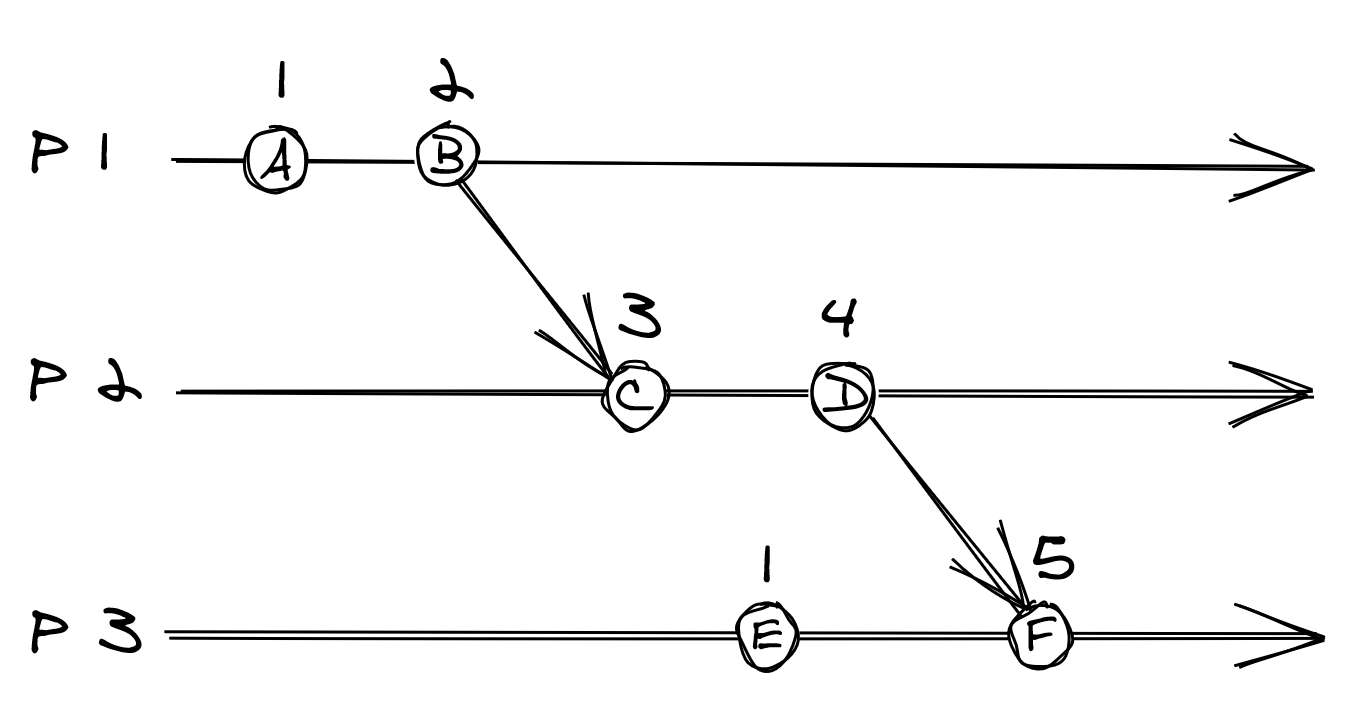
Figure 8.1: Three processes using Lamport clocks. For example, because D happened before F, D’s logical timestamp is less than F’s.

The Lamport clock assumes a crash-stop model, but a crash-recovery one can be supported by persisting the clock’s state on disk, for example.

The rules guarantee that if operation $O_1$ happened-before operation $O_2$, the logical timestamp of $O_1$ is less than the one of $O_2$. In the example shown in Figure 8.1, operation D happened-before F and their logical timestamps, 4 and 5, reflect that.

You would think that the converse also applies — if the logical timestamp of operation $O_3$ is less than $O_4$, then $O_3$ happened-before $O_4$. But, that can’t be guaranteed with Lamport timestamps. Going back to the example in Figure 8.1, operation E didn’t happen-before C, even if their timestamps seem to imply it. To guarantee the converse relationship, we will have to use a different type of logical clock: the vector clock.

8.3 Vector clocks

A vector clock is a logical clock that guarantees that if two operations can be ordered by their logical timestamps, then one must have happened-before the other. A vector clock is implemented with an array of counters, one for each process in the system. And similarly to how Lamport clocks are used, each process has its own local copy of the clock.

For example, if the system is composed of 3 processes $P1$, $P2$, and $P3$, each process has a local vector clock implemented with an array1 of 3 counters $[C_{P1}, C_{P2}, C_{P3}]$. The first counter in the array is associated with $P1$, the second with $P2$, and the third with $P3$.

A process updates its local vector clock based on the following rules:

• Initially, the counters in the array are set to 0.
• When an operation occurs, the process increments its own counter in the array by one.
• When the process sends a message, it increments its own counter in the array by one and sends a copy of the array with the message.
• When the process receives a message, it merges the array it received with the local one by taking the maximum of the two arrays element-wise. Finally, it increments its own counter in the array by one.

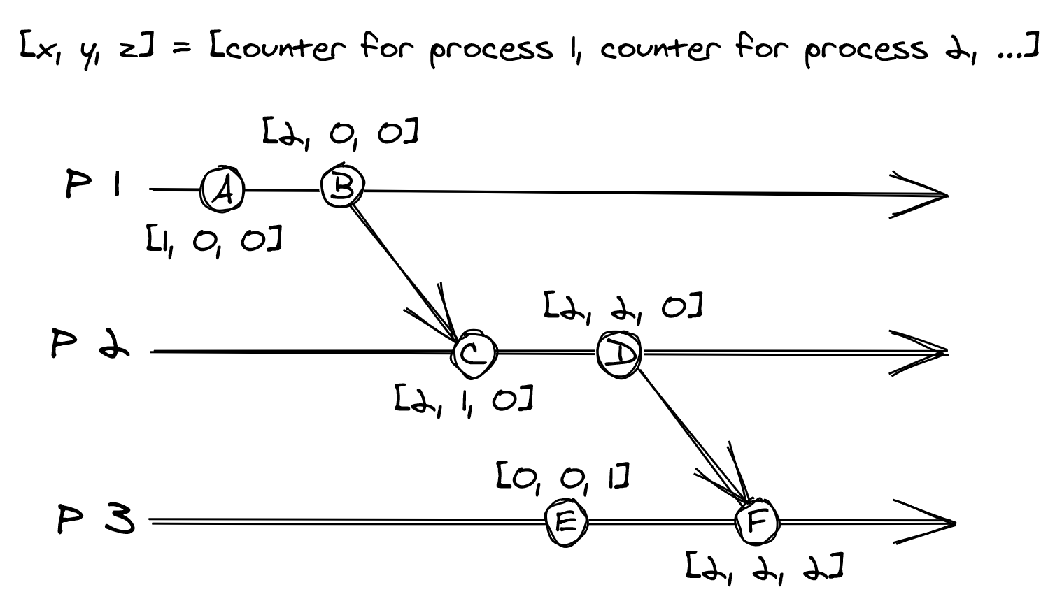
Figure 8.2: Each process has a vector clock represented with an array of three counters.

The beauty of vector clock timestamps is that they can be partially ordered; given two operations $O_1$ and $O_2$ with timestamps $T_1$ and $T_2$, if:

• every counter in $T_1$ is less than or equal the corresponding counter in $T_2$,
• and there is at least one counter in $T_1$ that is strictly less than the corresponding counter in $T_2$,

then $O_1$ happened-before $O_2$. For example, in Figure 8.2, B happened-before C.

If $O_1$ didn’t happen before $O_2$ and $O_2$ didn’t happen before $O_1$, then the timestamps can’t be ordered, and the operations are considered to be concurrent. For example, operation E and C in Figure 8.2 can’t be ordered, and therefore they are considered to be concurrent.

This discussion about logical clocks might feel quite abstract. Later in the book, we will encounter some practical applications of logical clocks. Once you learn to spot them, you will realize they are everywhere, as they can be disguised under different names. What’s important to internalize at this point is that generally, you can’t use physical clocks to derive accurately the order of events that happened on different processes2 .