1 Introduction
A distributed system is one in which the failure of a computer you didn’t even know existed can render your own computer unusable.
– Leslie Lamport
Loosely speaking, a distributed system is composed of nodes that cooperate to achieve some task by exchanging messages over communication links. A node can generically refer to a physical machine (e.g., a phone) or a software process (e.g., a browser).
Why do we bother building distributed systems in the first place?
Some applications are inherently distributed. For example, the web is a distributed system you are very familiar with. You access it with a browser, which runs on your phone, tablet, desktop, or Xbox. Together with other billions of devices worldwide, it forms a distributed system.
Another reason for building distributed systems is that some applications require high availability and need to be resilient to single-node failures. Dropbox replicates your data across multiple nodes so that the loss of a single node doesn’t cause all your data to be lost.
Some applications need to tackle workloads that are just too big to fit on a single node, no matter how powerful. For example, Google receives hundreds of thousands of search requests per second from all over the globe. There is no way a single node could handle that.
And finally, some applications have performance requirements that would be physically impossible to achieve with a single node. Netflix can seamlessly stream movies to your TV with high resolutions because it has a datacenter close to you.
This book will guide you through the fundamental challenges that need to be solved to design, build and operate distributed systems: communication, coordination, scalability, resiliency, and operations.
1.1 Communication
The first challenge comes from the fact that nodes need to communicate over the network with each other. For example, when your browser wants to load a website, it resolves the server’s address from the URL and sends an HTTP request to it. In turn, the server returns a response with the content of the page to the client.
How are request and response messages represented on the wire? What happens when there is a temporary network outage, or some faulty network switch flips a few bits in the messages? How can you guarantee that no intermediary can snoop into the communication?
Although it would be convenient to assume that some networking library is going to abstract all communication concerns away, in practice it’s not that simple because abstractions leak, and you need to understand how the stack works when that happens.
1.2 Coordination
Another hard challenge of building distributed systems is coordinating nodes into a single coherent whole in the presence of failures. A fault is a component that stopped working, and a system is fault-tolerant when it can continue to operate despite one or more faults. The “two generals” problem is a famous thought experiment that showcases why this is a challenging problem.
Suppose there are two generals (nodes), each commanding its own army, that need to agree on a time to jointly attack a city. There is some distance between the armies, and the only way to communicate is by sending a messenger (messages). Unfortunately, these messengers can be captured by the enemy (network failure).
Is there a way for the generals to agree on a time? Well, general 1 could send a message with a proposed time to general 2 and wait for a response. What if no response arrives, though? Was one of the messengers captured? Perhaps a messenger was injured, and it’s taking longer than expected to arrive at the destination? Should the general send another messenger?
You can see that this problem is much harder than it originally appeared. As it turns out, no matter how many messengers are dispatched, neither general can be completely certain that the other army will attack the city at the same time. Although sending more messengers increases the general’s confidence, it never reaches absolute certainty.
Because coordination is such a key topic, the second part of this book is dedicated to distributed algorithms used to implement coordination.
1.3 Scalability
The performance of a distributed system represents how efficiently it handles load, and it’s generally measured with throughput and response time. Throughput is the number of operations processed per second, and response time is the total time between a client request and its response.
Load can be measured in different ways since it’s specific to the system’s use cases. For example, number of concurrent users, number of communication links, or ratio of writes to reads are all different forms of load.
As the load increases, it will eventually reach the system’s capacity — the maximum load the system can withstand. At that point, the system’s performance either plateaus or worsens, as shown in Figure 1.1. If the load on the system continues to grow, it will eventually hit a point where most operations fail or timeout.
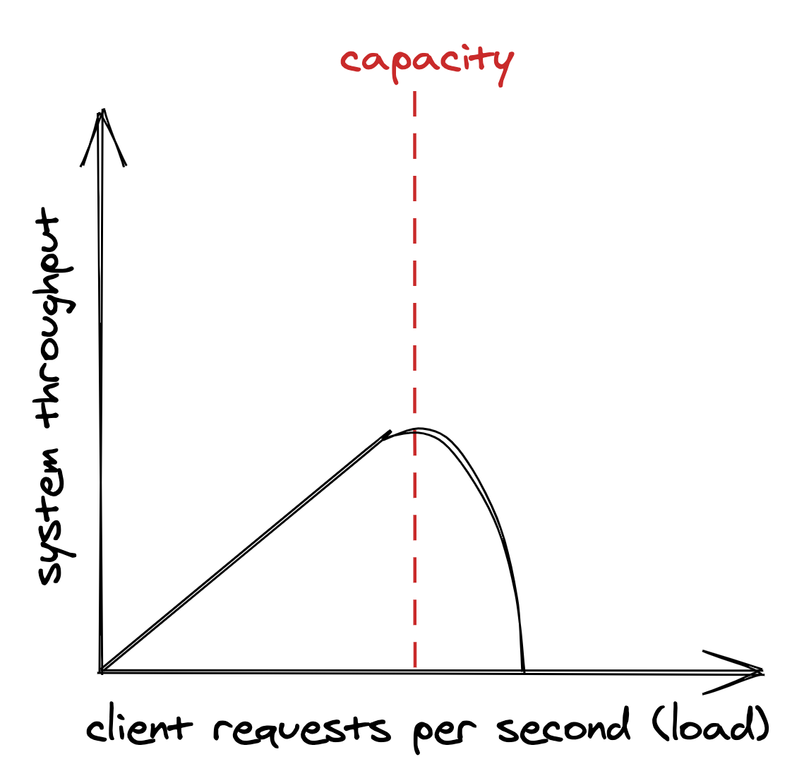
Figure 1.1: The system throughput on the y axis is the subset of client requests (x axis) that can be handled without errors and with low response times, also referred to as its goodput.
The capacity of a distributed system depends on its architecture and an intricate web of physical limitations like the nodes’ memory size and clock cycle, and the bandwidth and latency of network links.
A quick and easy way to increase the capacity is buying more expensive hardware with better performance, which is referred to as scaling up. But that will hit a brick wall sooner or later. When that option is no longer available, the alternative is scaling out by adding more machines to the system.
In the book’s third part, we will explore the main architectural patterns that you can leverage to scale out applications: functional decomposition, duplication, and partitioning.
1.4 Resiliency
A distributed system is resilient when it can continue to do its job even when failures happen. And at scale, any failure that can happen will eventually occur. Every component of a system has a probability of failing — nodes can crash, network links can be severed, etc. No matter how small that probability is, the more components there are, and the more operations the system performs, the higher the absolute number of failures becomes. And it gets worse, since failures typically are not independent, the failure of a component can increase the probability that another one will fail.
Failures that are left unchecked can impact the system’s availability, which is defined as the amount of time the application can serve requests divided by the duration of the period measured. In other words, it’s the percentage of time the system is capable of servicing requests and doing useful work.
Availability is often described with nines, a shorthand way of expressing percentages of availability. Three nines are typically considered acceptable, and anything above four is considered to be highly available.
| Availability % | Downtime per day |
|---|---|
| 90% (“one nine”) | 2.40 hours |
| 99% (“two nines”) | 14.40 minutes |
| 99.9% (“three nines”) | 1.44 minutes |
| 99.99% (“four nines”) | 8.64 seconds |
| 99.999% (“five nines”) | 864 milliseconds |
If the system isn’t resilient to failures, which only increase as the application scales out to handle more load, its availability will inevitably drop. Because of that, a distributed system needs to embrace failure and work around it using techniques such as redundancy and self-healing mechanisms.
As an engineer, you need to be paranoid and assess the risk that a component can fail by considering the likelihood of it happening and its resulting impact when it does. If the risk is high, you will need to mitigate it. Part 4 of the book is dedicated to fault tolerance and it introduces various resiliency patterns, such as rate limiting and circuit breakers.
1.5 Operations
Distributed systems need to be tested, deployed, and maintained. It used to be that one team developed an application, and another was responsible for operating it. The rise of microservices and DevOps has changed that. The same team that designs a system is also responsible for its live-site operation. That’s a good thing as there is no better way to find out where a system falls short than experiencing it by being on-call for it.
New deployments need to be rolled out continuously in a safe manner without affecting the system’s availability. The system needs to be observable so that it’s easy to understand what’s happening at any time. Alerts need to fire when its service level objectives are at risk of being breached, and a human needs to be looped in. The book’s final part explores best practices to test and operate distributed systems.
1.6 Anatomy of a distributed system
Distributed systems come in all shapes and sizes. The book anchors the discussion to the backend of systems composed of commodity machines that work in unison to implement a business feature. This comprises the majority of large scale systems being built today.
Before we can start tackling the fundamentals, we need to discuss the different ways a distributed system can be decomposed into parts and relationships, or in other words, its architecture. The architecture differs depending on the angle you look at it.
Physically, a distributed system is an ensemble of physical machines that communicate over network links.
At run-time, a distributed system is composed of software processes that communicate via inter-process communication (IPC) mechanisms like HTTP, and are hosted on machines.
From an implementation perspective, a distributed system is a set of loosely-coupled components that can be deployed and scaled independently called services.
A service implements one specific part of the overall system’s capabilities. At the core of its implementation is the business logic, which exposes interfaces used to communicate with the outside world. By interface, I mean the kind offered by your language of choice, like Java or C#. An “inbound” interface defines the operations that a service offers to its clients. In contrast, an “outbound” interface defines operations that the service uses to communicate with external services, like data stores, messaging services, and so on.
Remote clients can’t just invoke an interface, which is why adapters are required to hook up IPC mechanisms with the service’s interfaces. An inbound adapter is part of the service’s Application Programming Interface (API); it handles the requests received from an IPC mechanism, like HTTP, by invoking operations defined in the inbound interfaces. In contrast, outbound adapters implement the service’s outbound interfaces, granting the business logic access to external services, like data stores. This is illustrated in Figure 1.2.
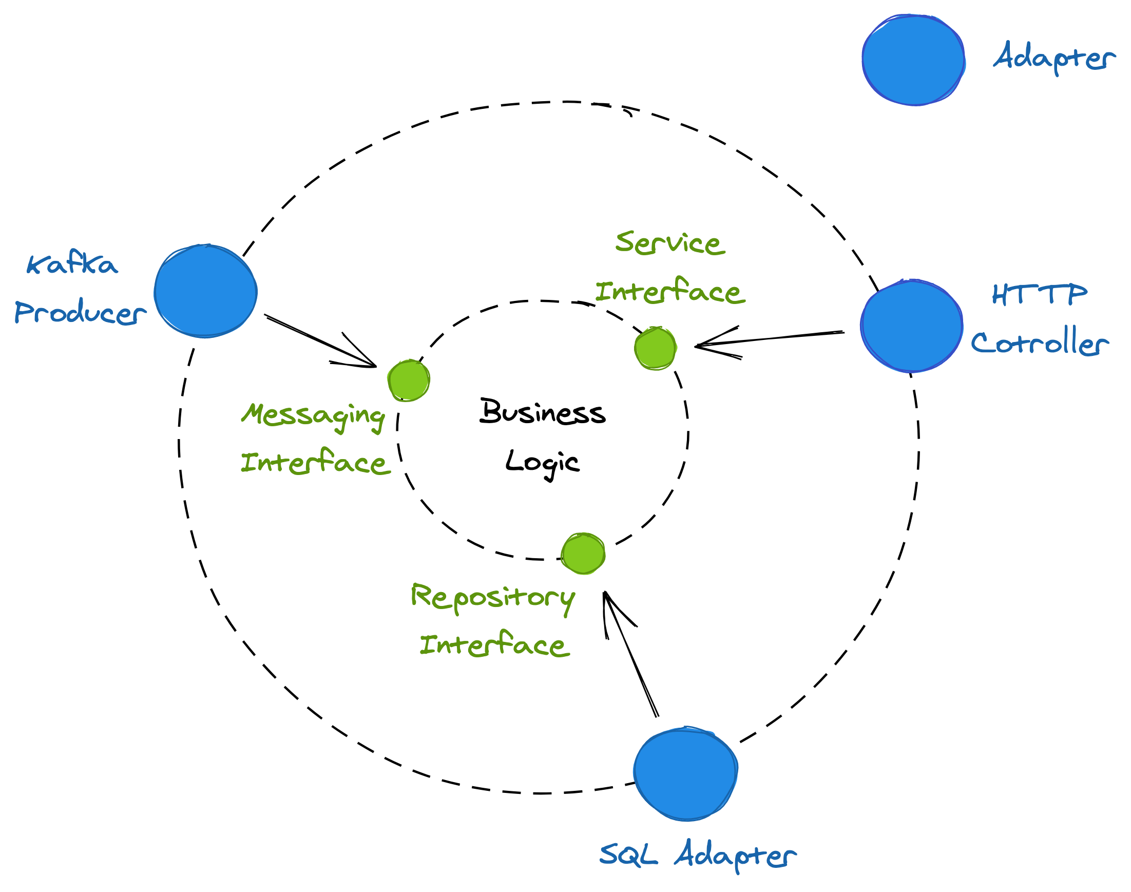
Figure 1.2: The business logic uses the messaging interface implemented by the Kafka producer to send messages and the repository interface to access the SQL store. In contrast, the HTTP controller handles incoming requests using the service interface.
A process running a service is referred to as a server, while a process that sends requests to a server is referred to as a client. Sometimes, a process is both a client and a server, since the two aren’t mutually exclusive.
For simplicity, I will assume that an individual instance of a service runs entirely within the boundaries of a single server process. Similarly, I assume that a process has a single thread. This allows me to neglect some implementation details that only complicate our discussion without adding much value.
In the rest of the book, I will switch between the different architectural points of view (see Figure 1.3), depending on which one is more appropriate to discuss a particular topic. Remember that they are just different ways to look at the same system.
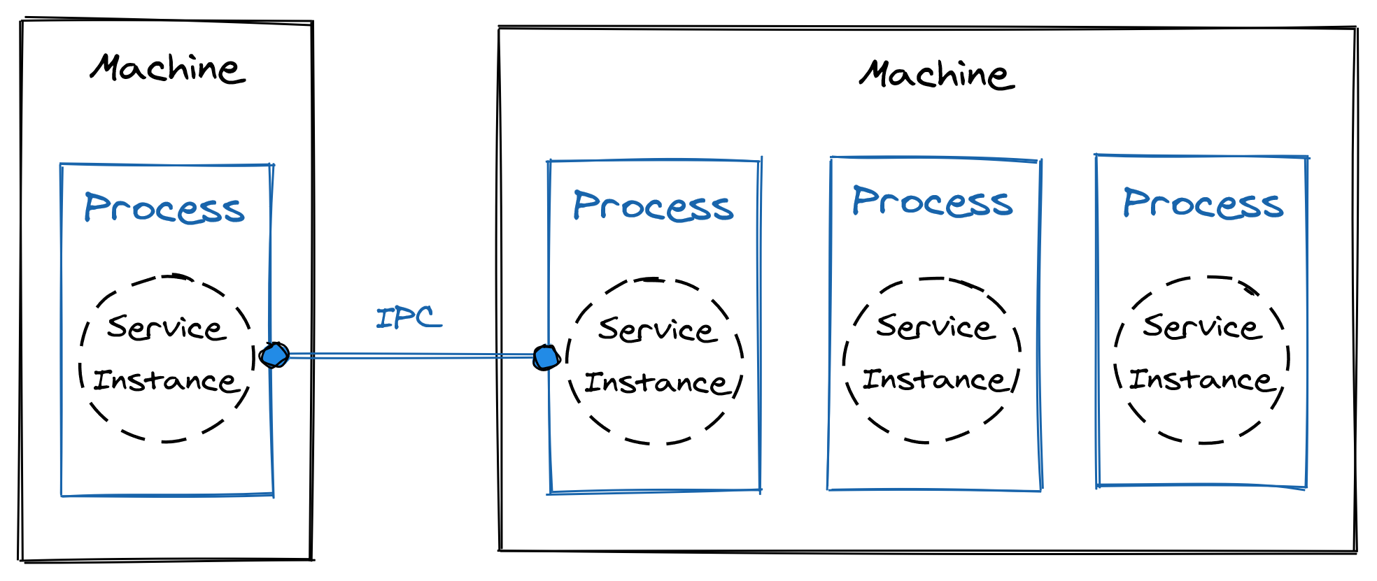
Figure 1.3: The different architectural points of view used in this book.