Chapter 30. Constantine’s Equivalence
I remember as a young programmer hearing dire reports that as much as 70% of software development costs went into maintenance. Seventy percent! How poor a job must we be doing that we make a thing and then have to spend twice as much just keeping it working?
Turns out that mental model of software, as a thing that is made and then should run forever unchanged, like some kind of perpetual motion machine, is the opposite of what really happens, and what should happen, too. The future value of a system reveals itself in today’s realities, not yesterday’s speculation.
With the way that coupling affects software development in place, we are ready to understand coupling’s significance. In the original work on coupling and cohesion, Structured Design, Ed Yourdon and Larry Constantine postulated that the goal of software design is to minimize the cost of software (it’s also to maximize the value, but we’ll get to that). But what are those costs?
That 70% estimate turns out to be way too low. If we apply our creativity, we can release value-creating software after only a few percent of its eventual development cost. It’s in everyone’s best interest to do so. The sooner we get feedback from real usage, the less time/money/opportunity we spend on behavior that doesn’t matter.
The first term of what I’ve dubbed “Constantine’s Equivalence,” then, is that the cost of software is approximately equal to the cost of changing it. Yes there is a brief period before we can be said to be “changing” it, but who cares? That period is economically insignificant. So:
cost(software) ~= cost(change)
Another way to think about this is graphically. (What follows is not actual data, just another way to think about the problem. Adjust accordingly.)
If we graph the cumulative cost of software over its lifespan, we get something like a logistic curve (Figure 30-1). The period before release represents both a small portion of the total time and a small portion of the total cost.
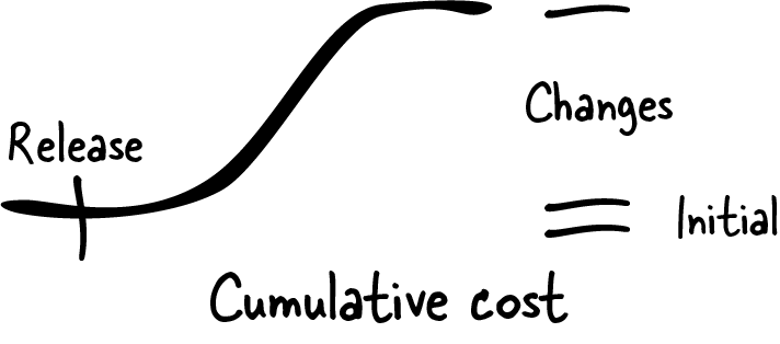
Figure 30-1. Logistic curve of cumulative cost showing that changes are most of the expense
What can we say about the cost of change? Are all changes equal? Of course not, not if I ask the question like that. We can bump along making small changes to the behavior of the system, all of them costing about the same. Then one day we make a change superficially similar to all the previous changes, but this one blows up in our faces. Instead of costing one unit, it costs ten or a hundred or a thousand.
Visualized, the cost per month (say) starts low, grows rapidly, then shrinks as other opportunities become more profitable (Figure 30-2). But why is the slope of cost growth so much steeper after release? Are we really making more changes? Yes, some more. But also, the existing system has started to create friction. We have to worry about backward compatibility. We have to worry about production stability. We have to worry about all the ways any one change might break seemingly unrelated features.
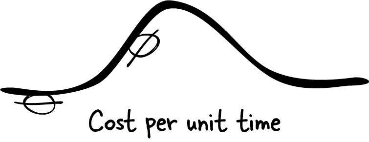
Figure 30-2. Cost per time grows slowly, then rapidly, then shrinks
If you know about power law distributions, you recognize what’s going on here (if you don’t know about power law distributions, please be careful, because I ended up obsessed by them for 20 years). One characteristic of power law distributions is that the few big “outlier” events matter a lot. Add them up and they outweigh the far more numerous “normal” events. The five biggest storms cause more damage than ten thousand small storms.
Is this sounding familiar? The most expensive behavior changes cost, together, far more than all the least expensive behavior changes put together. Put another way, the cost of change is approximately equal to the cost of the big changes:
cost(change) ~= cost(big changes)
What makes those expensive changes expensive? It’s when changing this element requires changing those two elements, each of which requires changing other elements, and… and… and…. What “propagates” change? Coupling. So, the cost of software is approximately equal to the coupling:
cost(big changes) ~= coupling
And now we have the full Constantine’s Equivalence:
cost(software) ~= cost(change) ~= cost(big changes) ~= coupling
Or, to highlight the importance of software design:
cost(software) ~= coupling
To reduce the cost of software, we must reduce coupling. But decoupling isn’t free and is subject to trade-offs, which we explore next.