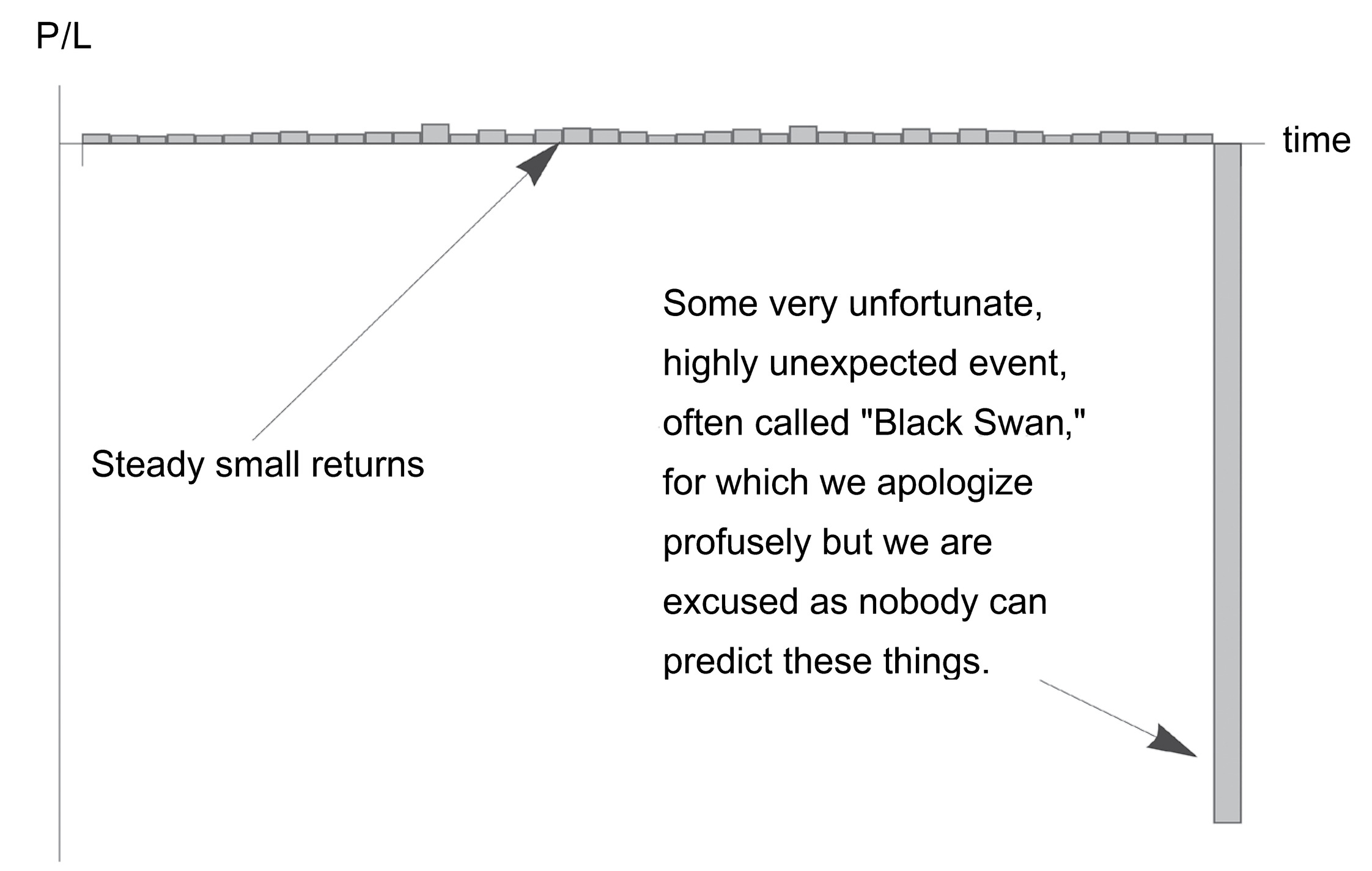
FIGURE 7. The Bob Rubin trade. Payoff in a skewed domain where the benefits are visible (and rewarded with some compensation) and the detriment is rare (and unpunished owing to absence of skin in the game). Can be generalized to politics, anything where the penalty is weak.

A. SKIN IN THE GAME AND TAIL PROBABILITIES

This section will analyze the probabilistic mismatch of tail risks and returns in the presence of a principal-agent problem.

Transfer of Harm: If an agent has the upside of the payoff of the random variable, with no downside, and is judged solely on the basis of past performance, then the incentive is to hide risks in the left tail using a negatively skewed (or more generally, asymmetric) distribution for the performance. This can be generalized to any payoff for which one does not bear the full risks and negative consequences of one’s actions.

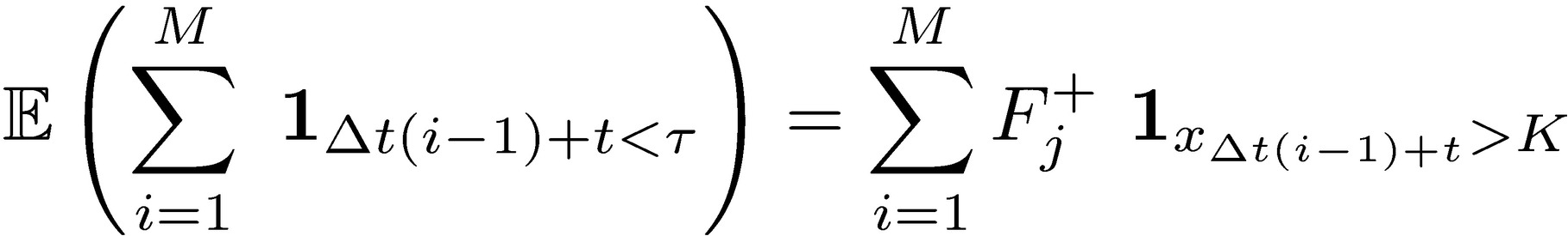
Let P(K, M) be the payoff for the operator over M incentive periods:

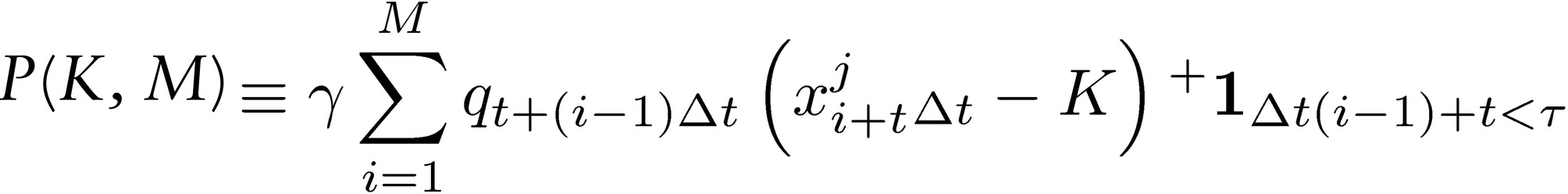
where 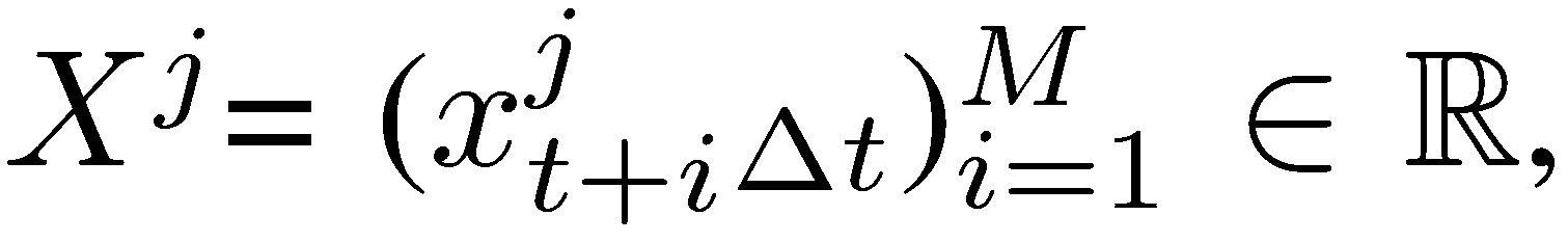i.i.d. random variables representing the distribution of profits over a certain period [t, t + iΔt], i ∈ ℕ, Δt ∈ ℝ⁺ and K is a “hurdle,” 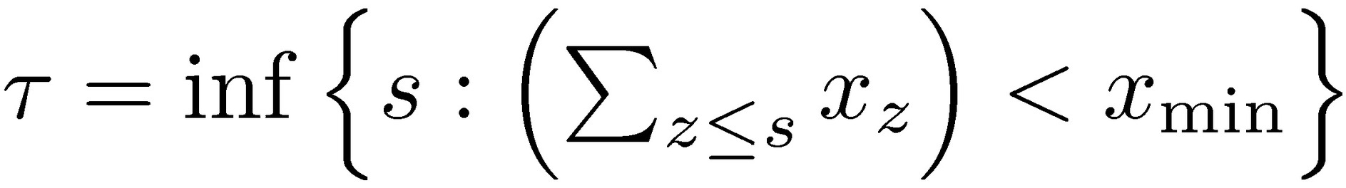is an indicator of stopping time when past performance conditions are not satisfied (namely, the condition of having a certain performance in a certain number of the previous years, otherwise the stream of payoffs terminates, the game ends and the number of positive incentives stops). The constant 𝛾 ∈ (0,1) is an “agent payoff,” or compensation rate from the performance, which does not have to be monetary (as long as it can be quantified as “benefit”). The quantity 𝑞_{𝑡+(𝑖−𝟷)Δ𝑡} ∈ [1,∞) indicates the size of the exposure at times t+(i-1 ) Δt (because of an Ito lag, as the performance at period s is determined by q at a strictly earlier period < s).

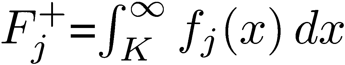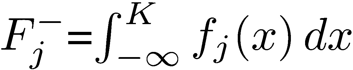Let {𝑓_j} be the family of probability measures 𝑓_j of X^j, 𝑗 ∈ ℕ. Each measure corresponds to certain mean/skewness characteristics, and we can split their properties in half on both sides of a “centrality” parameter K, as the “upper” and “lower” distributions. We write 𝑑𝐹_j(𝑥) as 𝑓_j(𝑥)𝑑𝑥, so and , the “upper” and “lower” distributions, each corresponding to certain conditional expectation 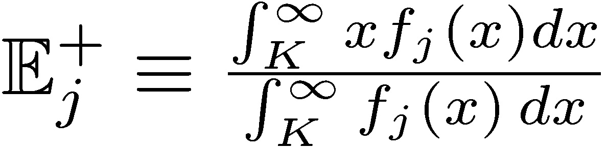and .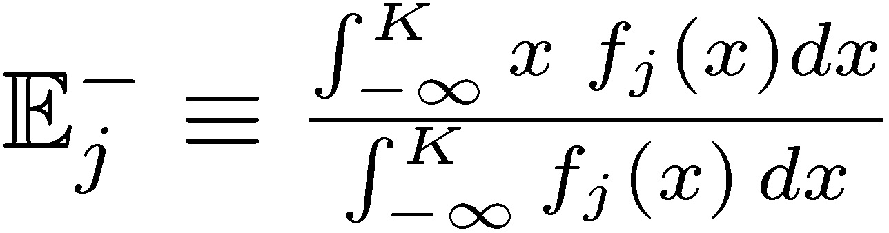

Now define 𝓿 ∈ ℝ⁺ as a K-centered nonparametric measure of asymmetry, , with values >1 for positive asymmetry, and <1 for negative ones. Intuitively, skewness has probabilities and expectations moving in opposite directions: the larger the negative payoff, the smaller the probability to compensate.

We do not assume a “fair game,” that is, with unbounded returns 𝑚 ∈ (-∞, ∞), F_j⁺ 𝔼_j⁺ + F_j⁻ 𝔼_j⁻ = m, which we can write as m⁺+m⁻= m.

Simplified assumptions of constant q and single-condition stopping time

Assume q constant, q = 1 and simplify the stopping time condition as having no loss in the previous periods, =inf{(𝑡+(𝑖-1)Δ𝑡)): 𝑥_Δ𝑡₍_𝑖−₁₎₊_𝑡 <𝐾} , which leads to

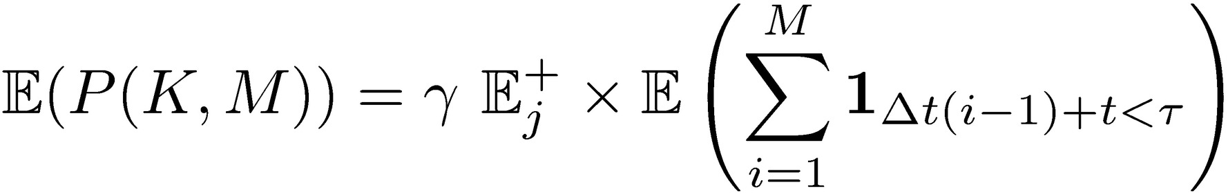
Since assuming independent and identically distributed agent’s payoffs, the expectation at stopping time corresponds to the expectation of stopping time multiplied by the expected compensation to the agent 𝛾 𝔼_j⁺. And .

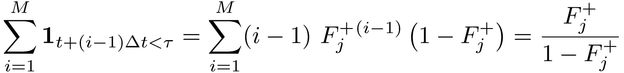
The expectation of stopping time can be written as the probability of success under the condition of no previous loss:

We can express the stopping time condition in terms of uninterrupted success runs. Let Σ be the ordered set of consecutive success runs Σ 𝄘 {{F }, {SF}, {SSF},…, {(M − 1) consecutive S, F}}, where S is success and F is failure over period Δt, with associated corresponding probabilities {(1 − F_j⁺), F_j⁺ (1 − F_j⁺), F_j⁺² (1−F_j⁺) ,…., F_j⁺^M⁻¹ (1⁻F_j⁺)},

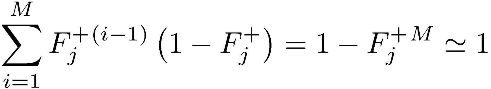
For M large, since F_j⁺ ∈ (0,1) we can treat the previous as almost an equality, hence:

Finally, the expected payoff for the agent:

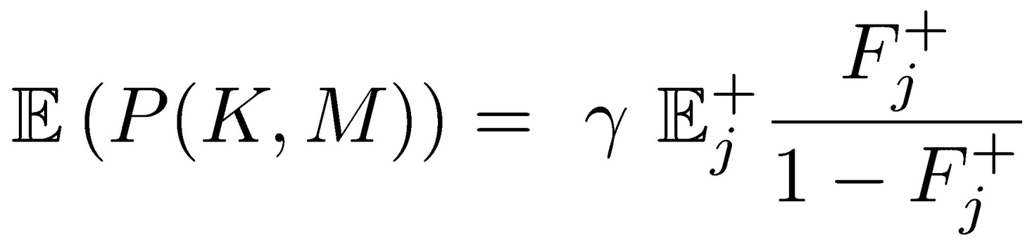
which increases by (i) increasing 𝔼_j⁺, (ii) minimizing the probability of the loss F_j⁻, but, and that’s the core point, even if (i) and (ii) take place at the expense of 𝑚, the total expectation from the package.

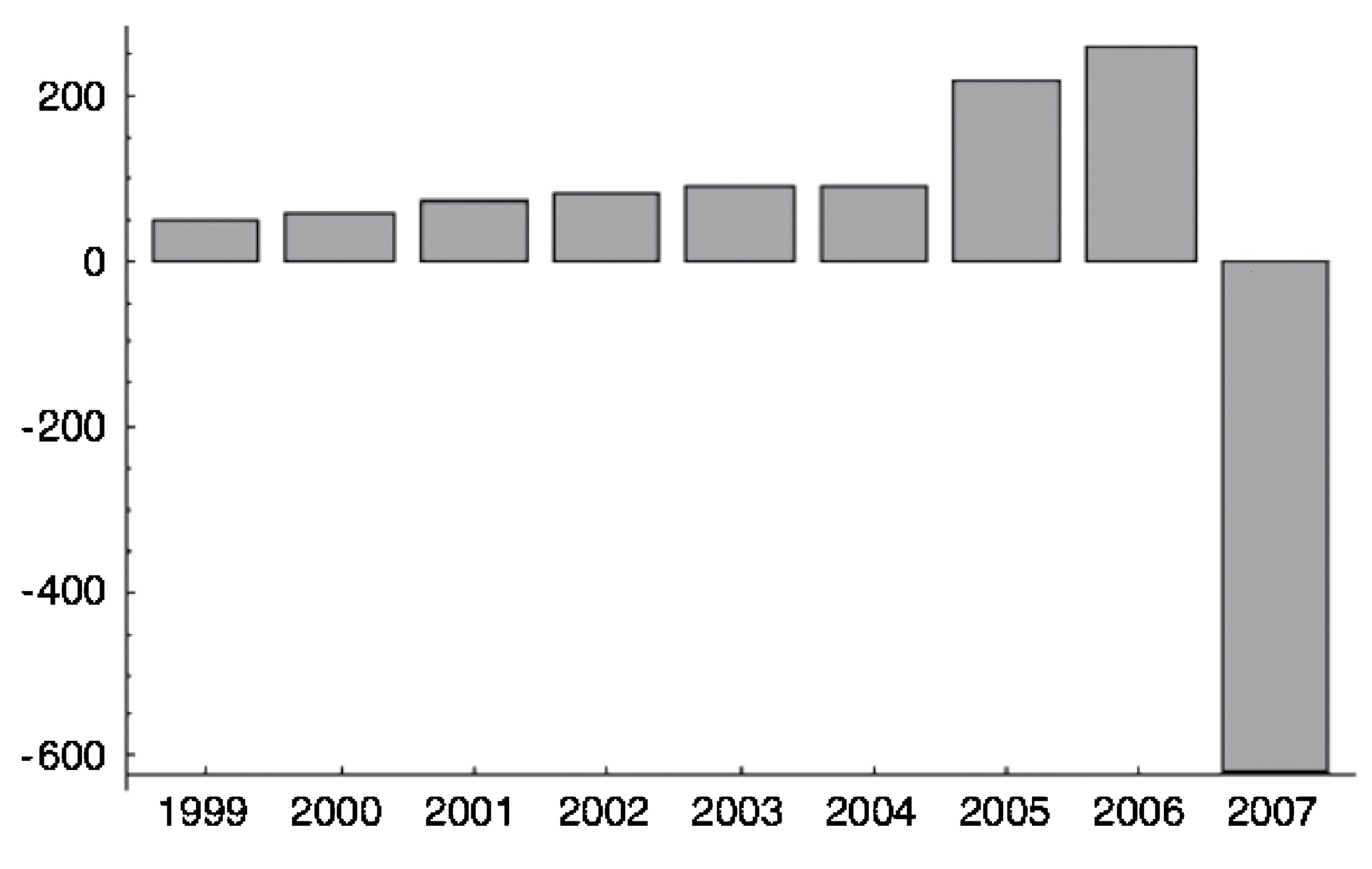
FIGURE 8. Indy Mac, a failed firm during the subprime crisis (from Taleb 2009). It is a representative of risks that keep increasing in the absence of losses, until explosive blowup.

Alarmingly, since , the agent doesn’t care about a degradation of the total expected return 𝑚 if it comes from the left side of the distribution, 𝑚⁻. Seen in skewness space, the expected agent payoff maximizes under the distribution 𝑗 with the lowest value of 𝓿_j (maximal negative asymmetry). The total expectation of the positive-incentive without-skin-in-the-game depends on negative skewness, not on 𝑚.

B. PROBABILISTIC SUSTAINABILITY AND ERGODICITY

Dynamic Risk Taking: If you take the risk—any risk—repeatedly, the way to count is in exposure per lifespan, or in the way it shortens the remaining lifespan.

Ruin Properties: Ruin probabilities are in the time domain for a single agent and do not correspond to state-space (or ensemble) tail probabilities. Nor are expectations fungible between the two domains. Statements on the “overestimation” of tail events (entailing ruin) by agents that are derived from state-space estimations are accordingly flawed. Many theories of “rationality” of agents are based on wrong estimation operators and/or probability measures.

This is the main reason behind the barbell strategy.

This is a special case of the conflation between a random variable and the payoff of a time-dependent, path-dependent derivative function.

Less Technical Translation:

Never cross a river if it is on average only 4 feet deep.*1

A simplified general case

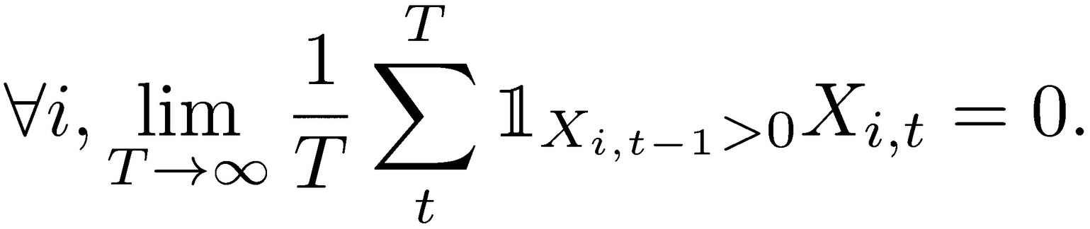
Consider the extremely simplified example, the sequence of independent random variables with support in the positive real numbers (ℝ⁺). The convergence theorems of classical probability theory address the behavior of the sum or average: lim 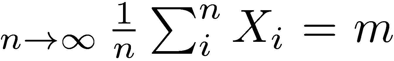by the (weak) law of large numbers (convergence in probability). As shown in the story of the casino in Chapter 19, n going to infinity produces convergence in probability to the true mean return m. Although the law of large numbers applies to draws i that can be strictly separated by time, it assumes (some) independence, and certainly path independence.

Now consider where every state variable X_i is indexed by a unit of time t : 0 < t < T. Assume that the “time events” are drawn from the exact same probability distribution: P(X_i) = P(X_i,t).

We define a time probability the evolution over time for a single agent i.

In the presence of terminal, that is irreversible, ruin, every observation is now conditional on some attribute of the preceding one, and what happens at period t depends on t − 1, what happens at t − 1 depends on t − 2, etc. We now have path dependence.

Next what we call failure of ergodicity:

Theorem 1 (state space-time inequality): Assume that ∀𝑡, 𝑃(𝑋_t = 0) > 0 and 𝑋₀ > 0, 𝔼_Ν(𝑋_𝑡) < ∞ the state space expectation for a static initial period t, and 𝔼_𝑇(𝑋_𝑖) the time expectation for any agent i, both obtained through the weak law of large numbers. We have

𝔼_Ν(𝑋_𝑡) ≥ 𝔼_𝑇(𝑋_𝑖)

Proof:

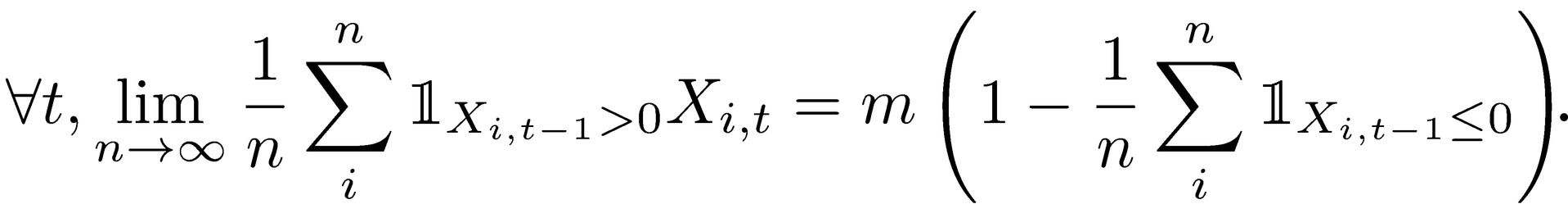
where 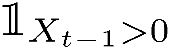is the indicator function requiring survival at the previous period. Hence the limits of n for t show a decreasing temporal expectation: 𝔼_Ν(𝑋_𝑡−1) ≤ 𝔼_Ν(𝑋_𝑡).

We can actually prove divergence.

As we can see by making T < ∞, by recursing the law of iterated expectations, we get the inequality for all T.

We can see the ensemble of risk takers expecting a return m in any period t, while every single risk taker is guaranteed to eventually go bust.

Other approaches: we can also approach the proof more formally in a measure-theoretic way by showing that while space sets for “nonruin” 𝓐 are disjoint, time sets are not. The approach relies on the fact that for a measure 𝓿:

does not necessarily equal

Almost all papers discussing the actuarial “overestimation” of tail risk via options (see review in Barberis 2003) are void by the inequality in Theorem 1. Clearly they assume that an agent only exists for a single decision or exposure. Simply, the original papers documenting the “bias” assume that the agents will never ever again make another decision in their remaining lives.

The usual solution to this path dependence—if it depends on only ruin—is done by introducing a function of X to allow the ensemble (path independent) average to have the same properties as the time (path dependent) average—or survival conditioned mean. The natural logarithm seems a good candidate. Hence log(X_i) and log(X_t) belong to the same probabilistic class; hence a probability measure on one is invariant with respect to the other—what is called ergodicity. In that sense, when analyzing performance and risk, under conditions of ruin, it is necessary to use a logarithmic transformation of the variable (Peters 2011), or boundedness of the left tail (Kelly 1956), while maximizing opportunity in the right tail (Gell-Mann 2016), or boundedness of the left tail (Geman et al. 2015).

What we showed here is that unless one takes a logarithmic transformation (or a similar—smooth—function producing −∞ with ruin set at X = 0), both expectations diverge. The entire point of the precautionary principle is to avoid having to rely on logarithms or transformations by reducing the probability of ruin.

In their magisterial paper, Peters and Gell-Mann (2014) showed that the Bernoulli use of the logarithm wasn’t for a concave “utility” function, but, as with the Kelly criterion, to restore ergodicity. A bit of history:

• Bernoulli discovers logarithmic risk taking under the illusion of “utility.”

• Kelly and Thorp recovered the logarithm for maximal growth criterion as an optimal gambling strategy. Nothing to do with utility.

• Samuelson disses logarithm as aggressive, not realizing that semi-logarithm (or partial logarithm), i.e., on partial of wealth, can be done. From Menger to Arrow, via Chernoff and Samuelson, many in decision theory are shown to be making the mistake of ergodicity.

• Pitman in 1975 shows that a Brownian motion subjected to an absorbing barrier at 0, with censored absorbing paths, becomes a three-dimensional Bessel process. The drift of the surviving paths is , which integrates to a logarithm.

• Peters and Gell-Mann recover the logarithm for ergodicity and, in addition, put the Kelly-Thorpe result on rigorous physical grounds.

• With Cirillo, this author (Taleb and Cirillo 2015) discovers the log as unique smooth transformation to create a dual of the distribution in order to remove one-tail compact support to allow the use of extreme value theory.

• We can show (Briys and Taleb, in progress and private communication) the necessity of logarithmic transformation as simple ruin avoidance, which happens to be a special case of the HARA utility class.

Adaptation of Theorem 1 to Brownian Motion

The implications of simplified discussion do not change whether one uses richer models, such as a full stochastic process subjected to an absorbing barrier. And of course in a natural setting the eradication of all previous life can happen (i.e., X_t can take extreme negative value), not just a stopping condition. The Peters and Gell-Mann argument also cancels the so-called equity premium puzzle if you add fat tails (hence outcomes vastly more severe pushing some level equivalent to ruin) and absence of the fungibility of temporal and ensemble. There is no puzzle.

The problem is invariant in real life if one uses a Brownian-motion-style stochastic process subjected to an absorbing barrier. In place of the simplified representation we would have, for an process subjected to L, an absorbing barrier from below, in the arithmetic version:

otherwise

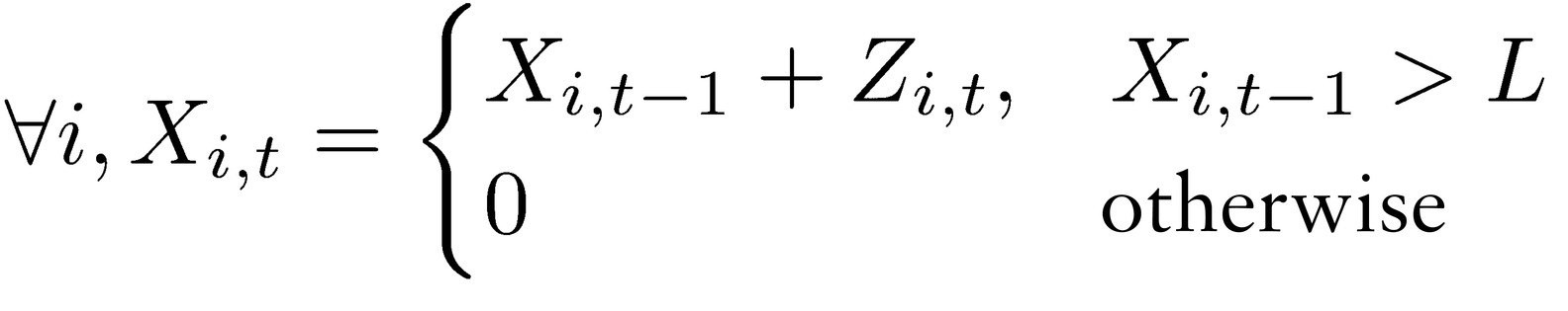
or, for a geometric process:

otherwise

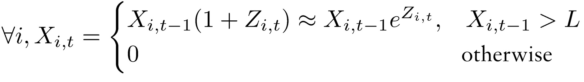
where Z is a random variable.

Going to continuous time, and considering the geometric case, let ={inf 𝑡 : 𝑋_i,t > 𝐿}be the stopping time. The idea is to have the simple expectation of the stopping time match the remaining lifespan—or remain in the same order.

We switched the focus from probability to the mismatch between stopping time for ruin and the remaining lifespan.

C. PRINCIPLE OF PROBABILISTIC SUSTAINABILITY

Principle: A unit needs to take any risk as if it were going to take it repeatedly—at a specified frequency—over its remaining lifespan.

The principle of sustainability is necessary for the following argument. While experiments are static (we saw the confusion between the state-space and the temporal), life is continuous. If you incur a tiny probability of ruin as a “one-off” risk, survive it, then do it again (another “one-off” deal), you will eventually go bust with probability 1. Confusion arises because it may seem that the “one-off” risk is reasonable, but that also means that an additional one is reasonable. (See Figure 9). The good news is that some classes of risk can be deemed to be practically of probability zero: the earth survived trillions of natural variations daily over three billion years, otherwise we would not be here. We can use conditional probability arguments (adjusting for the survivorship bias) to back-out the ruin probability in a system.

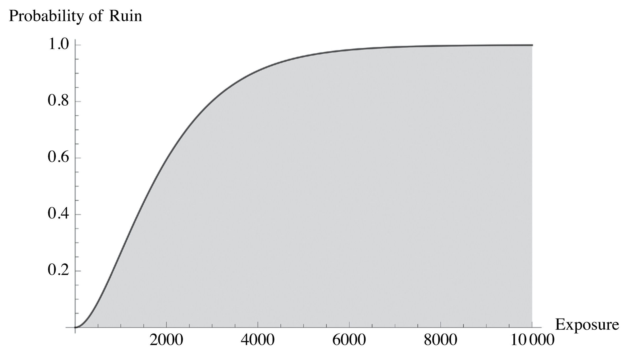
FIGURE 9. Why ruin is not a renewable resource. No matter how small the probability, in time, something bound to hit the ruin barrier is about guaranteed to hit it. No risk should be considered a “one-off” event.

Now, we do not have to take 𝑡 → ∞ nor is permanent sustainability necessary. We can just extend shelf time. The longer the t, the more the expectation operators diverge.

Consider the unconditional expected stopping time to ruin in a discrete and simplified model: , where is the number of exposures per time period, T is the overall remaining lifespan, and p is the ruin probability, both over that same time period for fixing p. Since , we can calibrate the risk under repetition. The longer the life expectancy T (expressed in time periods), the more serious the ruin problem. Humans and plants have a short shelf life, nature doesn’t—at least for t of the order of 10⁸ years—hence annual ruin probabilities of O(10⁻⁸) and (for tighter increments) local ruin probabilities of at most O(10⁻⁵⁰). The higher up in the hierarchy individual-species-ecosystem, the more serious the ruin problem. This duality hinges on 𝑡 → ∞; hence requirement is not necessary for items that are not permanent, that have a finite shelf life.

The fat tails argument: The more a system is capable of delivering large deviations, the worse the ruin problem.

We will cover the fat tails problem more extensively. Clearly the variance of the process matters; but overall deviations that do not exceed the ruin threshold do not matter.

Logarithmic transformation

Under the axiom of sustainability, i.e., that “one should take risks as if you were going to do it forever,” only a logarithmic (or similar) transformation applies.

Fattailedness is a property that is typically worrisome under absence of compact support for the random variable, less so when the variables are bounded. But as we saw the need of using a logarithmic transformation, a random variable with support in [0, ∞) now has support in (−∞, ∞), hence properties derived from extreme value theory can now apply to our analysis. Likewise, if harm is defined as a positive number with an upper bound H which corresponds to ruin, it is possible to transform it from [0, H] to [0, ∞).

Cramér and Lundberg, in insurance analysis, discovered the difficulty; see Cramér 1930.

A Note on Ergodicity^*2: Ergodicity is not statistically identifiable, not observable, and there is no test for time series that gives ergodicity, similar to Dickey-Fuller for stationarity (or Phillips-Perron for integration order). More crucially:

If your result is obtained from the observation of a time series, how can you make claims about the ensemble probability measure?

The answer is similar to arbitrage, which has no statistical test but, crucially, has a probability measure determined ex ante (the “no free lunch” argument). Further, consider the argument of a “self-financing” strategy, via, say, dynamic hedging. At the limit we assume that the law of large numbers will compress the returns and that no loss and no absorbing barrier will ever be reached. It satisfies our criterion of ergodicity but does not have a statistically obtained measure. Further, almost all the literature on intertemporal investments/consumption requires absence of ruin.

We are not asserting that a given security or random process is ergodic, but that, given that its ensemble probability (obtained by cross-sectional methods, assumed via subjective probabilities, or simply determined by arbitrage arguments), a risk-taking strategy should conform to such properties. So ergodicity concerns the function of the random variable or process, not the process itself. And the function should not allow ruin.

In other words, assuming the SP500 has a certain expected return “alpha,” an ergodic strategy would generate a strategy, say Kelly Criterion, to capture the assumed alpha. If it doesn’t, because of absorbing barrier or something else, it is not ergodic.

D. TECHNICAL DEFINITION OF FAT TAILS

Probability distributions range between extreme thin-tailed (Bernoulli) and extreme fat-tailed. Among the categories of distributions that are often distinguished due to the convergence properties of moments are: (1) Having a support that is compact but not degenerate, (2) Subgaussian, (3) Gaussian, (4) Subexponential, (5) Power law with exponent greater than 3, (6) Power law with exponent less than or equal to 3 and greater than 2, (7) Power law with exponent less than or equal to 2. In particular, power law distributions have a finite mean only if the exponent is greater than 1, and have a finite variance only if the exponent exceeds 2.

Our interest is in distinguishing between cases where tail events dominate impacts, as a formal definition of the boundary between the categories of distributions to be considered as Mediocristan and Extremistan. The natural boundary between these occurs at the subexponential class, which has the following property:

Let X = be a sequence of independent and identically distributed random variables with support in (ℝ⁺), with cumulative distribution function F. The subexponential class of distributions is defined by (see Teugels 1975, Pitman 1980):

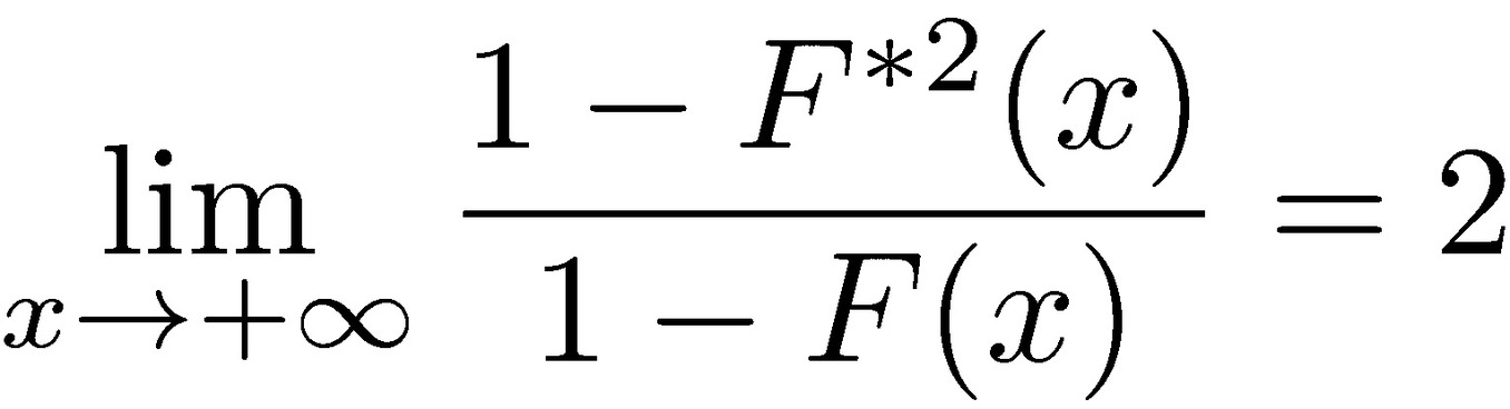
where 𝐹*² = 𝐹′ ∗ 𝐹 is the cumulative distribution of X₁ + X₂, the sum of two independent copies of X. This implies that the probability that the sum X₁ + X₂ exceeds a value x is twice the probability that either one separately exceeds x. Thus, every time the sum exceeds x, for large enough values of x, the value of the sum is due to either one or the other exceeding x—the maximum over the two variables—and the other of them contributes negligibly.

More generally, it can be shown that the sum of n variables is dominated by the maximum of the values over those variables in the same way. Formally, the following two properties are equivalent to the subexponential condition (see Chistyakov 1964, Embrechts et al. 1979). For a given n ≥ 2, let 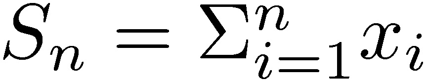and M_n = max

a) lim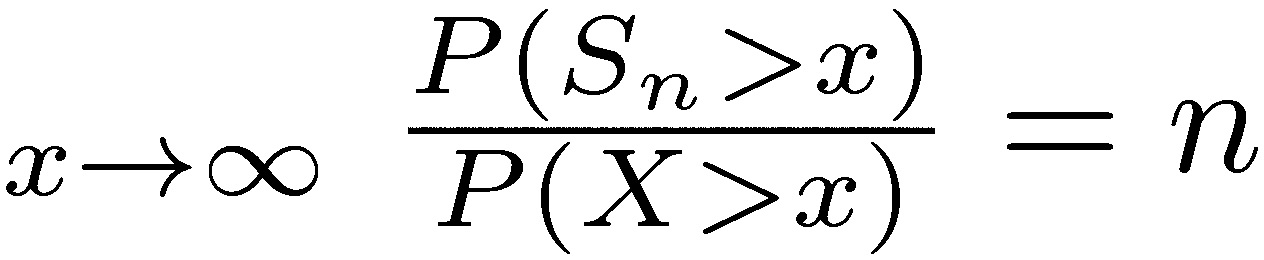

b) lim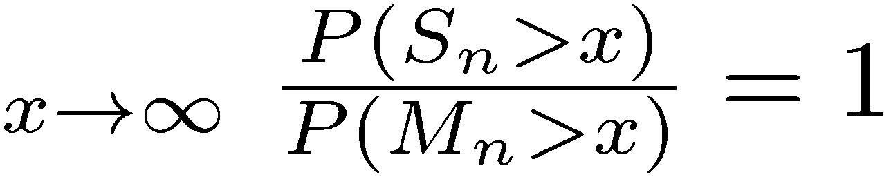

Thus the sum S_n has the same magnitude as the largest sample M_n, which is another way of saying that tails play the most important role.

Intuitively, tail events in subexponential distributions should decline more slowly than an exponential distribution for which large tail events should be irrelevant. Indeed, one can show that subexponential distributions have no exponential moments:

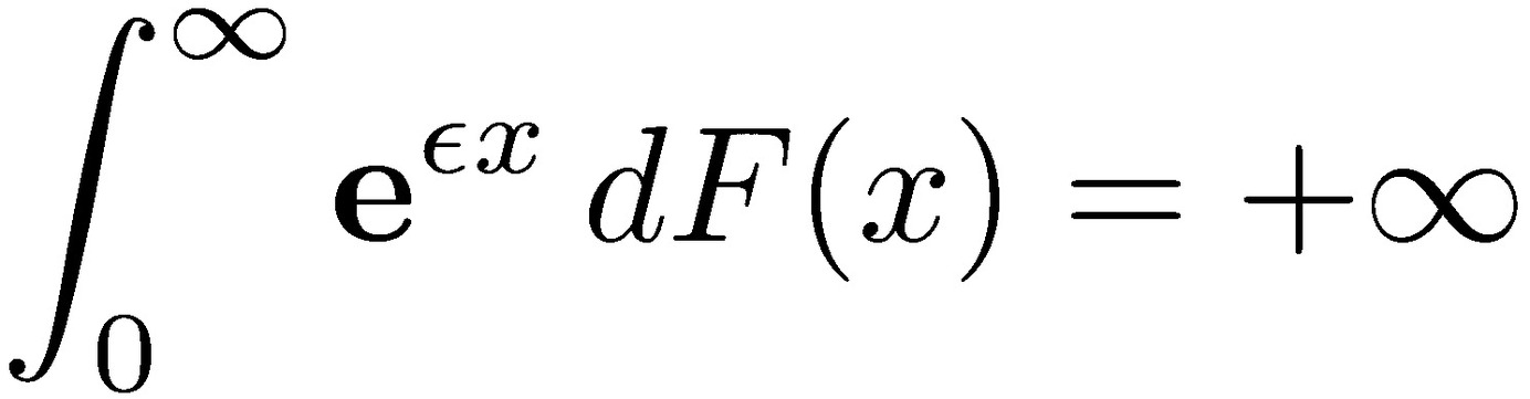
for all values of 𝜀 greater than zero. However, the converse isn’t true, since distributions can have no exponential moments, yet not satisfy the subexponential condition.

We note that if we choose to indicate deviations as negative values of the variable 𝑥, the same result holds by symmetry for extreme negative values, replacing 𝑥 → +∞ with 𝑥 → −∞. For two-tailed variables, we can separately consider positive and negative domains.