I started this book with the idea that readers who would get through most of the chapters would also be interested in the future of real-world cryptography. While you’re reading an applied and practical book with a focus on what is in use today, the field of cryptography is rapidly changing (as we saw in recent years with cryptocurrencies, for example).
As you’re reading this book, a number of theoretical cryptographic primitives and protocols are making their ways into the applied cryptography world—maybe because these theoretical primitives are finally finding a use case or because they’re finally becoming efficient enough to be used in real-world applications. Whatever the reason, the real world of cryptography is definitely growing and getting more exciting. In this chapter, I give you a taste of what the future of real-world cryptography might look like (perhaps in the next 10 to 20 years) by briefly introducing three primitives:
Secure multi-party computation (MPC)—A subfield of cryptography that allows different participants to execute a program together without necessarily revealing their own input to the program.
Fully homomorphic encryption (FHE)—The holy grail of cryptography, a primitive used to allow arbitrary computations on encrypted data.
General-purpose zero-knowledge proofs (ZKPs)—The primitive you learned about in chapter 7 that allows you to prove that you know something without revealing that something, but this time, applied more generally to more complex programs.
This chapter contains the most advanced and complicated concepts in the book. For this reason, I recommend that you glance at it and then move on to chapter 16 to read the conclusion. When you are motivated to learn more about the inners of these more advanced concepts, come back to this chapter. Let’s get started!
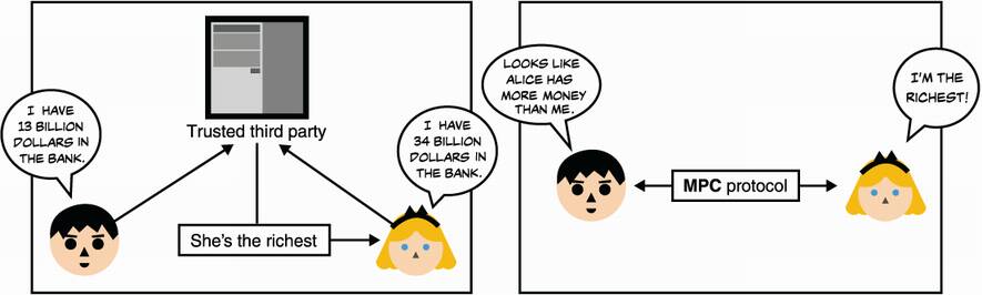
Secure multi-party computation (MPC) is a field of cryptography that came into existence in 1982 with the famous Millionaires’ problem. In his 1982 paper “Protocols for Secure Computations,” Andrew C. Yao wrote, “Two millionaires wish to know who is richer; however, they do not want to find out inadvertently any additional information about each other’s wealth. How can they carry out such a conversation?” Simply put, MPC is a way for multiple participants to compute a program together. But before learning more about this new primitive, let’s see why it’s useful.
We know that with the help of a trusted third party, any distributed computation can easily be worked out. This trusted third party can perhaps maintain the privacy of each participant’s input, as well as possibly restricting the amount of information revealed by the computation to specific participants. In the real world, though, we don’t like trusted third parties too much; we know that they are pretty hard to come by, and they don’t always respect their commitments.
MPC allows us to completely remove trusted third parties from a distributed computation and enables participants to compute the computation by themselves without revealing their respective inputs to one another. This is done through a cryptographic protocol. With that in mind, using MPC in a system is pretty much the equivalent to using a trusted third party (see figure 15.1).
Figure 15.1 A secure multi-party computation (MPC) protocol turns a distributed computation that can be calculated via a trusted third party (image on the left) into a computation that doesn’t need the help of a trusted third party (image on the right).
Note that you already saw some MPC protocols. Threshold signatures and distributed key generations, covered in chapter 8, are examples of MPC. More specifically, these examples are part of a subfield of MPC called threshold cryptography, which has been receiving a lot of love in more recent years with, for example, NIST in mid-2019 kicking off a standardization process for threshold cryptography.
Another well-known subfield of MPC is the field of private set intersection (PSI), which poses the following problem: Alice and Bob have a list of words, and they want to know which words (or perhaps just how many) they have in common without revealing their respective list of words. One way to solve this problem is to use the oblivious pseudorandom function (OPFR) construction you learned about in chapter 11. (I illustrate this protocol in figure 15.2.) If you recall
Alice obtains the random values, PRF(key, word), for every word in her list using the OPRF protocol (so she doesn’t learn the PRF key and Bob doesn’t learn the words).
Bob then can compute the list of PRF (key, word) values for his own words and send it to Alice, who is then able to compare it with her own PRF outputs to see if any of Bob’s PRF outputs matches.
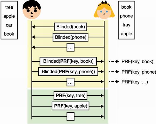
Figure 15.2 Private set intersection (PSI) allows Alice to learn what words she has in common with Bob. First, she blinds every word she has in her list and uses the OPRF protocol with Bob to apply a PRF using Bob’s key on each of her words. Finally, Bob sends her the PRF of his key with his words. Alice can then see if anything matches to learn what words they have in common.
PSI is a promising field that is starting to see more and more adoption in recent years, as it has shown to be much more practical than it used to be. For example, Google’s Password Checkup feature integrated into the Chrome browser uses PSI to warn you when some of your passwords have been detected in password dumps following password breaches without actually seeing your passwords. Interestingly, Microsoft also does this for its Edge browser but uses fully homomorphic encryption (which I’ll introduce in the next section) to perform the private set intersection. On the other hand, the developers of the Signal messaging application (discussed in chapter 10) decided that PSI was too slow to perform contact discovery in order to figure out who you can talk to based on your phone’s contact list, and instead, used SGX (covered in chapter 13) as a trusted third party.
More generally, MPC has many different solutions aiming at the computation of arbitrary programs. General-purpose MPC solutions all provide different levels of efficiency (from hours to milliseconds) and types of properties. For example, how many dishonest participants can the protocol tolerate? Are participants malicious or just honest but curious (also called semi-honest, a type of participant in MPC protocols that is willing to execute the protocol correctly but might attempt to learn the other participants’ inputs)? Is it fair to all participants if some of them terminate the protocol early?
Before a program can be securely computed with MPC, it needs to be translated into an arithmetic circuit. Arithmetic circuits are successions of additions and multiplications, and because they are Turing complete, they can represent any program! For an illustration of an arithmetic circuit, see figure 15.3.
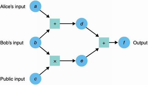
Figure 15.3 An arithmetic circuit is a number of addition or multiplication gates linking inputs to outputs. In the figure, values travel from left to right. For example, d = a + b. Here, the circuit only outputs one value f = a + b + bc, but it can in theory have multiple output values. Notice that different inputs to the circuit are provided by different participants, but they could also be public inputs (known to everyone).
Before taking a look at the next primitive, let me give you a simplified example of an (honest-majority) general-purpose MPC built via Shamir’s secret sharing. Many more schemes exist, but this one is simple enough to fit here in a three-step explanation: share enough information on each input in the circuit, evaluate every gate in the circuit, and reconstruct the output. Let’s look at each step in more detail.
The first step is for every participant to have enough information about each input of the circuit. Public inputs are shared publicly, while private inputs are shared via Shamir’s secret sharing (covered in chapter 8). I illustrate this in figure 15.4.
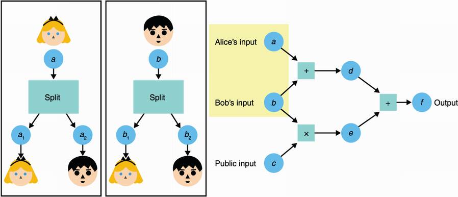
Figure 15.4 The first step of a general-purpose MPC with secret sharing is to have participants split their respective secret inputs (using Shamir’s secret sharing scheme) and distribute the parts to all participants. For example, here Alice splits her input a into a1 and a2. Because there are only two participants in this example, she gives the first share to herself and gives Bob the second one.
The second step is to evaluate every gate of the circuit. For technical reasons I’ll omit here, addition gates can be computed locally, while multiplication gates must be computed interactively (participants must exchange some messages). For an addition gate, simply add the input shares you have; for a multiplication gate, multiply the input shares. What you get is a share of the result as figure 15.5 illustrates. At this point, the shares can be exchanged (in order to reconstruct the output) or kept separate to continue the computation (if they represent an intermediate value).
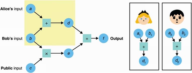
Figure 15.5 The second step of a general-purpose MPC with secret sharing is to have participants compute each gate in the circuit. For example, a participant can compute an addition gate by adding the two input Shamir shares that they have, which produces a Shamir share of the output.
The final step is to reconstruct the output. At this point, the participants should all own a share of the output, which they can use to reconstruct the final output using the final step of Shamir’s secret sharing scheme.
There’s been huge progress in the last decade to make MPC practical. It is a field of many different use cases, and one should be on the lookout for the potential applications that can benefit from this newish primitive. Note that, unfortunately, no real standardization effort exists, and while several MPC implementations can be considered practical for many use cases today, they are not easy to use.
Incidentally, the general-purpose MPC construction I explained earlier in this section is based on secret sharing, but there are more ways to construct MPC protocols. A well-known alternative is called garbled circuits, which is a type of construction first proposed by Yao in his 1982 paper introducing MPC. Another alternative is based on fully homomorphic encryption, a primitive you’ll learn about in the next section.
For a long time in cryptography, a question has troubled many cryptographers: is it possible to compute arbitrary programs on encrypted data? Imagine that you could encrypt the values a, b, and c separately, send the ciphertexts to a service, and ask that service to return the encryption of a × 3b + 2c + 3, which you could then decrypt. The important idea here is that the service never learns about your values and always deals with ciphertexts. This calculation might not be too useful, but with additions and multiplications, one can compute actual programs on the encrypted data.
This interesting concept, originally proposed in 1978 by Rivest, Adleman, and Dertouzos, is what we call fully homomorphic encryption (FHE) (or as it used to be called, the holy grail of cryptography). I illustrate this cryptographic primitive in figure 15.6.
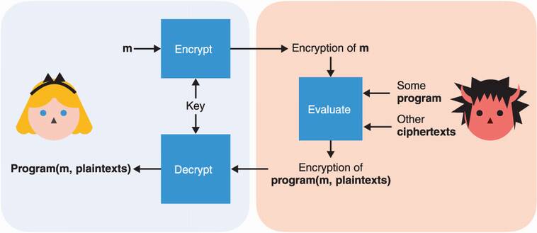
Figure 15.6 Fully homomorphic encryption (FHE) is an encryption scheme that allows for arbitrary computations over encrypted content. Only the owner of the key can decrypt the result of the computation.
By the way, you already saw some cryptographic schemes that should make you feel like you know what I’m talking about. Think of RSA (covered in chapter 6): given a ciphertext = messagee mod N, someone can easily compute some restricted function of the ciphertext
ne × ciphertext = (n × message)e mod N
for any number n they want (although it can’t be too big). The result is a ciphertext that decrypts to
Of course, this is not a desired behavior for RSA, and it has led to some attacks (for example, Bleichenbacher’s attack mentioned in chapter 6). In practice, RSA breaks the homomorphism property by using a padding scheme. Note that RSA is homomorphic only for the multiplication, which is not enough to compute arbitrary functions, as both multiplication and addition are needed for those. Due to this limitation, we say that RSA is partially homomorphic.
Other types of homomorphic encryptions include
Somewhat homomorphic—Which means partially homomorphic for one operation (addition or multiplication) and homomorphic for the other operation in limited ways. For example, additions are unlimited up to a certain number but only a few multiplications can be done.
Leveled homomorphic—Both addition and multiplication are possible up to a certain number of times.
Fully homomorphic—Addition and multiplication are unlimited (it’s the real deal).
Before the invention of FHE, several types of homomorphic encryption schemes were proposed, but none could achieve what fully homomorphic encryption promised. The reason is that by evaluating circuits on encrypted data, some noise grows; after a point, the noise has reached a threshold that makes decryption impossible. And, for many years, some researchers tried to prove that perhaps there was some information theory that could show that fully homomorphic encryption was impossible; that is, until it was shown to be possible.
One night, Alice dreams of immense riches, caverns piled high with silver, gold and diamonds. Then, a giant dragon devours the riches and begins to eat its own tail! She awakes with a feeling of peace. As she tries to make sense of her dream, she realizes that she has the solution to her problem.
—Craig Gentry (“Computing Arbitrary Functions of Encrypted Data,” 2009)
In 2009, Craig Gentry, a PhD student of Dan Boneh, proposed the first-ever fully homomorphic encryption construction. Gentry’s solution was called bootstrapping, which in effect was to evaluate a decryption circuit on the ciphertext every so often in order to reduce the noise to a manageable threshold. Interestingly, the decryption circuit itself does not reveal the private key and can be computed by the untrusted party. Bootstrapping allowed turning a leveled FHE scheme into an FHE scheme. Gentry’s construction was slow and quite impractical, reporting about 30 minutes per basic bit operation, but as with any breakthrough, it only got better with time. It also showed that fully homomorphic encryption was possible.
How does bootstrapping work? Let’s see if we can gain some insight. First, I need to mention that we’ll need not a symmetric encryption system, but a public key encryption system, where a public key can be used to encrypt and a private key can be used to decrypt. Now, imagine that you execute a certain number of additions and multiplications on a ciphertext and reach some level of noise. The noise is low enough to still allow you to decrypt the ciphertext correctly, but too high that it won’t let you perform more homomorphic operations without destroying the encrypted content. I illustrate this in figure 15.7.
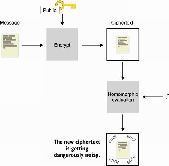
Figure 15.7 After encrypting a message with a fully homomorphic encryption algorithm, operating on it increases its noise to dangerous thresholds, where decryption becomes impossible.
You could think that you’re stuck, but bootstrapping unsticks you by removing the noise out of that ciphertext. To do that, you re-encrypt the noisy ciphertext under another public key (usually called the bootstrapping key) to obtain an encryption of that noisy ciphertext. Notice that the new ciphertext has no noise. I illustrate this in figure 15.8.
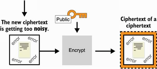
Figure 15.8 Building on figure 15.7, to eliminate the noise of the ciphertext, you can decrypt it. But because you don’t have the secret key, instead you re-encrypt the noisy ciphertext under another public key (called the bootstrapping key) to obtain a new ciphertext of a noisy ciphertext without error.
Now comes the magic: you are provided with the initial private key, not in cleartext, but encrypted under that bootstrapping key. This means that you can use it with a decryption circuit to homomorphically decrypt the inner noisy ciphertext. If the decryption circuit produces an acceptable amount of noise, then it works, and you will end up with the result of the first homomorphic operation encrypted under the bootstrapping key. I illustrate this in figure 15.9.
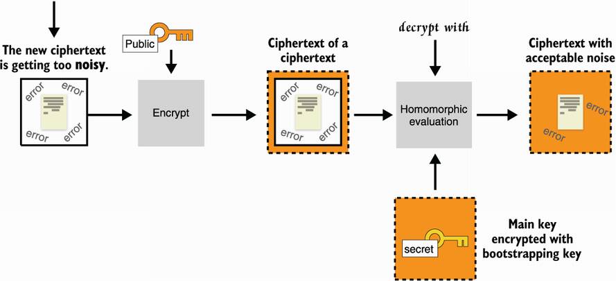
Figure 15.9 Building on figure 15.9, you use the initial secret key encrypted to the bootstrapping key to apply the decryption circuit to that new ciphertext. This effectively decrypts the noisy ciphertext in place, removing the errors. There will be some amount of errors due to the decryption circuit.
If the remaining amount of errors allows you to do at least one more homomorphic operation (+ or ×), then you are gold: you have a fully homomorphic encryption algorithm because you can always, in practice, run the bootstrapping after or before every operation. Note that you can set the bootstrapping key pair to be the same as the initial key pair. It’s a bit weird as you get some circular security oddity, but it seems to work and no security issues are known.
Before moving on, let’s see one example of an FHE scheme based on the learning with errors problem we saw in chapter 14. I’ll explain a simplified version of the GSW scheme, named after the authors Craig Gentry, Amit Sahai, and Brent Waters. To keep things simple, I’ll introduce a secret key version of the algorithm, but just keep in mind that it is relatively straightforward to transform such a scheme into a public key variant, which we need for bootstrapping. Take a look at the following equation where C is a square matrix, s is a vector, and m is a scalar (a number):
In this equation, s is called an eigenvector and m is an eigenvalue. If these words are foreign to you, don’t worry about it; they don’t matter much here.
The first intuition in our FHE scheme is obtained by looking at the eigenvectors and eigenvalues. The observation is that if we set m to a single bit we want to encrypt, C to be the ciphertext, and s to be the secret key, then we have an (insecure) homomorphic encryption scheme to encrypt one bit. (Of course, we assume there is a way to obtain a random ciphertext C from a fixed bit m and a fixed secret key s.) I illustrate this in figure 15.10 in a Lego kind of way.
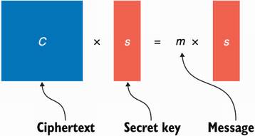
Figure 15.10 We can produce an insecure homomorphic encryption scheme to encrypt a single bit m with a secret vector s by interpreting m as an eigenvalue and s as an eigenvector and then finding the associated matrix C, which will be the ciphertext.
To decrypt a ciphertext, you multiply the matrix with the secret vector s and see if you obtain the secret vector back or 0. You can verify that the scheme is fully homomorphic by checking that the decryption of two ciphertexts added together (C1 + C2) results in the associated bits added together:
(C1 + C2)s = C1s + C2s = b1s + b2s = (b1 + b2)s
Also, the decryption of two ciphertexts multiplied together (C1 × C2) results in the associated bits multiplied together:
(C1 × C2)s = C1 (C2s) = C1 (b2s) = b2C1s = (b2 × b1) s
Unfortunately, that scheme is insecure as it is trivial to retrieve the eigenvector (the secret vector s) from C. What about adding a bit of noise? We can change this equation a bit to make it look like our learning with errors problem:
This should look more familiar. Again, we can verify that the addition is still homomorphic:
(C1 + C2)s = C1s + C2s = b1s + e1 + b2s + e2 = (b1 + b2)s + (e1+e2)
Here, notice that the error is growing (e1 + e2), which is what we expected. We can also verify that the multiplication is still working as well:
(C1 × C2)s = C1 (C2s) = C1 (b2s + e2) = b2C1s + C1e2 = b2 (b1s + e1) + C1e2
= (b2 × b1) s + b2e1 + C1e2
Here, b2e1 is small (as it is either e1 or 0), but C1e2 is potentially large. This is obviously a problem, which I’m going to ignore to avoid digging too much into the details. If you’re interested in learning more, make sure to read Shai Halevi’s “Homomorphic Encryption” report (2017), which does an excellent job at explaining all of these things and more.
The most touted use case of FHE has always been the cloud. What if I could continue to store my data in the cloud without having it seen? And, additionally, what if the cloud could provide useful computations on that encrypted data? Indeed, one can think of many applications where FHE could be useful. A few examples include
A spam detector could scan your emails without looking at those.
Genetic research could be performed on your DNA without actually having to store and protect your privacy-sensitive human code.
A database could be stored encrypted and queried on the server side without revealing any data.
Yet Phillip Rogaway, in his seminal 2015 paper on “The Moral Character of Cryptographic Work,” notes that “FHE [. . .] have engendered a new wave of exuberance. In grant proposals, media interviews, and talks, leading theorists speak of FHE [. . .] as game-changing indications of where we have come. Nobody seems to emphasize just how speculative it is that any of this will ever have any impact on practice.”
While Rogaway is not wrong, FHE is still quite slow, advances in the field have been exciting. At the time of this writing (2021), operations are about one billion times slower than normal operations, yet since 2009, there has been a 109 speed-up. We are undoubtedly moving towards a future where FHE will be possible for at least some limited applications.
Furthermore, not every application needs the full-blown primitive; somewhat homomorphic encryption can also be used in a wide range of applications and is much more efficient than FHE. A good indicator that a theoretical cryptography primitive is entering the real world is standardization, and indeed, FHE is no foreigner to that. The https://homomorphicencryption.org standardization effort includes many large companies and universities. It is still unclear exactly when, where, and in what form homomorphic encryption will make its entry into the real world. What’s clear is that it will happen, so stay tuned!
I talked about zero-knowledge proofs (ZKPs) in chapter 7 on signatures. There, I pointed out that signatures are similar to non-interactive ZKPs of knowledge for discrete logarithms. These kinds of ZKPs were invented in the mid-1980s by Professors Shafi Goldwasser, Silvio Micali, and Charles Rackoff. Shortly after, Goldreich, Micali, and Wigderson found that we could prove much more than just discrete logarithms or other types of hard problems; we could also prove the correct execution of any program even if we removed some of the inputs or outputs (see figure 15.11 for an example). This section focuses on this general-purpose type of ZKP.
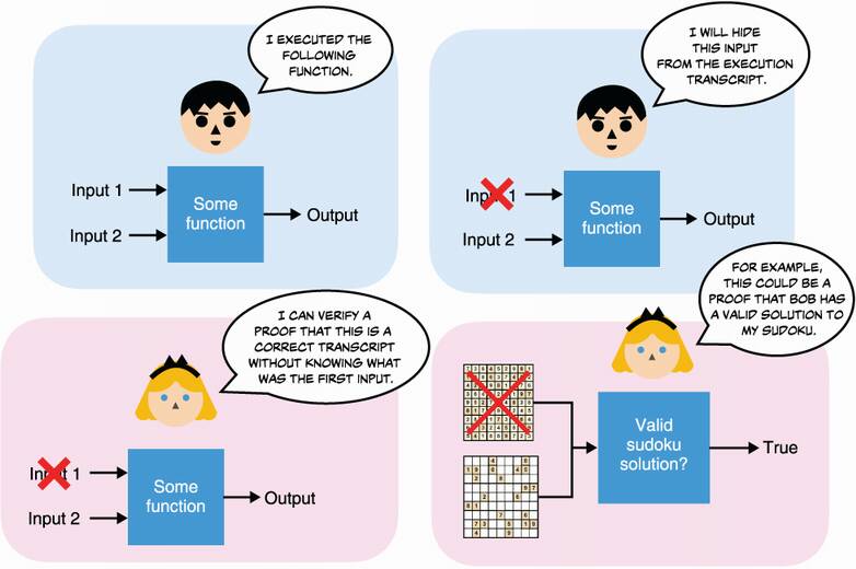
Figure 15.11 General-purpose ZKPs allow a prover to convince a verifier about the integrity of an execution trace (the inputs of a program and the outputs obtained after its execution) while hiding some of the inputs or outputs involved in the computation. An example of this is a prover trying to prove that a sudoku can be solved.
ZKP as a field has grown tremendously since its early years. One major reason for this growth is the cryptocurrency boom and the need to provide more confidentiality to on-chain transactions as well as optimize on space. The field of ZKP is still growing extremely fast as of the time of this writing, and it is quite hard to follow what are all the modern schemes that exist and what types of general-purpose ZKPs there are.
Fortunately for us, this problem was getting large enough that it tripped the standardization threshold, an imaginary line that, when reached, almost always ends up motivating some people to work together towards a clarification of the field. In 2018, actors from the industry and academia joined together to form the ZKProof Standardization effort with the goal to “standardize the use of cryptographic zero-knowledge proofs.” To this day, it is still an ongoing effort. You can read more about it at https://zkproof.org.
You can use general-purpose ZKPs in quite a lot of different situations, but to my knowledge, they have mostly been used in the cryptocurrency space so far, probably due to the high number of people interested in cryptography and willing to experiment with the bleeding edge stuff. Nonetheless, general-purpose ZKPs have potential applications in a lot of fields: identity management (being able to prove your own age without revealing it), compression (being able to hide most of a computation), confidentiality (being able to hide parts of a protocol), and so on. The biggest blockers for more applications to adopt general-purpose ZKPs seem to be the following:
The large number of ZKP schemes and the fact that every year more schemes are being proposed.
The difficulty of grasping how these systems work and how to use them for specific use cases.
Distinctions between the different proposed schemes are quite important. Because it is a great source of confusion, here is how some of these schemes are divided:
Zero-knowledge or not—If some of the information needs to remain secret from some of the participants, then we need zero-knowledgeness. Note that proofs without secrets can be useful as well. For example, you might want to delegate some intensive computation to a service that, in turn, has to prove to you that the result they provide is correct.
Interactive or not—Most ZKP schemes can be made non-interactive (sometimes using the Fiat-Shamir transformation I talked about in chapter 7), and protocol designers seem most interested in the non-interactive version of the scheme. This is because back-and-forth’s can be time consuming in protocols, but also because interactivity is sometimes not possible. So-called non-interactive proofs are often referred to as NIZKs for non-interactive ZKPs.
Succinct proofs or not—Most of the ZKP schemes in the spotlight are often referred to as zk-SNARKs for Zero-Knowledge Succinct Non-Interactive Argument of Knowledge. While the definition can vary, it focuses on the size of the proofs produced by such systems (usually in the order of hundreds of bytes), and the amount of time needed to verify them (within the range of milliseconds). zk-SNARKs are, thus, short and easy to use to verify ZKPs. Note that a scheme not being a zk-SNARK does not disqualify it for the real world as often different properties might be useful in different use cases.
Transparent setup or not—Like every cryptographic primitive, ZKPs need a setup to agree on a set of parameters and common values. This is called a common reference string (CRS). But setups for ZKPs can be much more limiting or dangerous than initially thought. There are three types of setup:
Quantum-resistant or not—Some ZKPs make use of public key cryptography and advanced primitives like bilinear pairings (which I’ll explain later), while others only rely on symmetric cryptography (like hash functions), which makes them naturally resistant to quantum computers (usually at the expense of much larger proofs).
Because zk-SNARKs are what’s up at the time of this writing, let me give you my perception as to how they work.
First and foremost, there are many, many zk-SNARK schemes—too many of them, really. Most build on this type of construction:
A proving system, allowing a prover to prove something to a verifier.
A translation or compilation of a program to something the proving system can prove.
The first part is not too hard to understand, while the second part sort of requires a graduate course in the subject. To begin, let’s take a look at the first part.
The main idea of zk-SNARKs is that they are all about proving that you know some polynomial f(x) that has some roots. By roots I mean that the verifier has some values in mind (for example, 1 and 2) and the prover must prove that the secret polynomial they have in mind evaluates to 0 for these values (for example, f(1) = f(2) = 0). By the way, a polynomial that has 1 and 2 as roots (as in our example) can be written as f(x) = (x – 1)(x – 2)h(x) for some polynomial h(x). (If you’re not convinced, try to evaluate that at x = 1 and x = 2.) We say that the prover must prove that they know an f(x) and h(x) such that f(x) = t(x)h(x) for some target polynomial t(x) = (x – 1)(x – 2). In this example, 1 and 2 are the roots that the verifier wants to check.
But that’s it! That’s what zk-SNARKs proving systems usually provide: something to prove that you know some polynomial. I’m repeating this because the first time I learned about that it made no sense to me. How can you prove that you know some secret input to a program if all you can prove is that you know a polynomial? Well, that’s why the second part of a zk-SNARK is so difficult. It’s about translating a program into a polynomial. But more on that later.
Back to our proving system, how does one prove that they know such a function f(x)? They have to prove that they know an h(x) such that you can write f(x) as f(x) = t(x)h(x). Ugh, ... not so fast here. We’re talking about zero-knowledge proofs right? How can we prove this without giving out f(x)? The answer is in the following three tricks:
Homomorphic commitments—A commitment scheme similar to the ones we used in other ZKPs (covered in chapter 7)
Bilinear pairings—A mathematical construction that has some interesting properties; more on that later
The fact that different polynomials evaluate to different values most of the time
So let’s go through each of these, shall we?
The first trick is to use commitments to hide the values that we’re sending to the prover. But not only do we hide them, we also want to allow the verifier to perform some operations on them so that they can verify the proof. Specifically, they need to verify that if the prover commits on their polynomial f(x) as well as h(x), then we have
com(f(x)) = com(t(x)) com(h(x)) = com(t(x)h(x))
where the commitment com(t(x)) is computed by the verifier as the agreed constraint on the polynomial. These operations are called homomorphic operations, and we couldn’t have performed them if we had used hash functions as commitment mechanisms (as mentioned in chapter 2). Thanks to these homomorphic commitments, we can “hide values in the exponent” (for example, for a value v, send the commitment gv mod p) and perform useful identity checks:
The equality of commitments—The equality ga = gb means that a = b
The addition of commitments—The equality ga = gbgc means that a = b + c
The scaling of commitments—The equality ga = (gb)c means that a = bc
Notice that the last check only works if c is a public value and not a commitment (gc). With homomorphic commitments alone we can’t check the multiplication of commitments, which is what we needed. Fortunately, cryptography has another tool to get such equations hidden in the exponent—bilinear pairings.
Bilinear pairings can be used to unblock us, and this is the sole reason why we use bilinear pairings in a zk-SNARK (really, just to be able to multiply the values inside the commitments). I don’t want to go too deep into what bilinear pairings are, but just know that it is another tool in our toolkit that allows us to multiply elements that couldn’t be multiplied previously by moving them from one group to another.
Using e as the typical way of writing a bilinear pairing, we have e(g1, g2) = h3, where g1, g2, and h3 are generators for different groups. Here, we’ll use the same generator on the left (g1 = g2) which makes the pairing symmetric. We can use a bilinear pairing to perform multiplications hidden in the exponent via this equation:
Again, we use bilinear pairings to make our commitments not only homomorphic for the addition, but also for the multiplication. (Note that this is not a fully homomorphic scheme as multiplication is limited to a single one.) Bilinear pairings are also used in other places in cryptography and are slowly becoming a more common building block. They can be seen in homomorphic encryption schemes and also signatures schemes like BLS (which I mentioned in chapter 8).
Finally, the succinctness of zk-SNARKs comes from the fact that two functions that differ evaluate to different points most of the time. What does this mean for us? Let’s say that I don’t have a polynomial f(x) that really has the roots we’ve chosen with the verifier, this means that f(x) is not equal to t(x)h(x). Then, evaluating f(x) and t(x)h(x) at a random point r won’t return the same result most of the time. For almost all r, f(r)≠ t(r)h(r). This is known as the Schwartz-Zippel lemma, which I illustrate in figure 15.12.
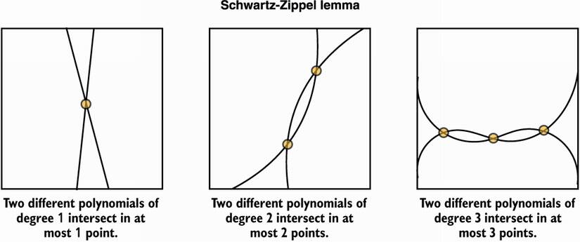
Figure 15.12 The Schwartz-Zippel lemma says that two different polynomials of degree n can intersect in at most n points. In other words, two different polynomials will differ in most points.
Knowing this, it is enough to prove that com(f(r)) = com(t(r)h(r)) for some random point r. This is why zk-SNARK proofs are so small: by comparing points in a group, you end up comparing much larger polynomials. But this is also the reason behind the trusted setup needed in most zk-SNARK constructions. If a prover knows the random point r that will be used to check the equality, then they can forge an invalid polynomial that will still verify the equality. So a trusted setup is about
Committing different exponentiations of r (for example, g, gr, gr2, gr3, . . .) so that these values can be used by the prover to compute their polynomial without knowing the point r
Does the second point make sense? If my polynomial as the prover is f(x) = 3x2 + x + 2, then all I have to do is compute (gr2)3 gr g2 to obtain a commitment of my polynomial evaluated at that random point r (without knowing r).
So far, the constraints on the polynomial that the prover must find is that it needs to have some roots: some values that evaluate to 0 with our polynomial. But how do we translate a more general statement into a polynomial knowledge proof? Typical statements in cryptocurrencies, which are the applications currently making the most use of zk-SNARKs these days, are of the form:
Prove that a value is in the range [0, 264] (this is called a range proof)
Prove that a (secret) value is included in some given (public) Merkle tree
Prove that the sum of some values is equal to the sum of some other values
And herein lies the difficult part. As I said earlier, converting a program execution into the knowledge of a polynomial is really hard. The good news is that I’m not going to tell you all about the details, but I’ll tell you enough to give you a sense of how things work. From there, you should be able to understand what are the parts that are missing from my explanation and fill in the gaps as you wish. What is going to happen next is the following:
Our program will first get converted into an arithmetic circuit, like the ones we saw in the section on MPC.
That arithmetic circuit will be converted into a system of equations that are of a certain form (called a rank-1 constraint system or R1CS).
We then use a trick to convert our system of equations into a polynomial.
First, let’s assume that almost any program can be rewritten more or less easily in math. The reason why we would want to do that should be obvious: we can’t prove code, but we can prove math. For example, the following listing provides a function where every input is public except for a, which is our secret input.
Listing 15.1 A simple function
fn my_function(w, a, b) {
  if w == true {
    return a * (b + 3);
   } else {
    return a + b;
   }
}
In this simple example, if every input and output is public except for a, one can still deduce what a is. This listing also serves as an example of what you shouldn’t try to prove in zero-knowledge. Anyway, the program can be rewritten in math with this equation:
w × (a × (b + 3)) + (1 – w) × (a + b) = v
Where v is the output and w is either 0 (false) or 1 (true). Notice that this equation is not really a program or a circuit, it just looks like a constraint. If you execute the program correctly and then fill in the inputs and outputs obtained in the equation, the equality should be correct. If the equality is not correct, then your inputs and outputs don’t correspond to a valid execution of the program.
This is how you have to think about these general-purpose ZKPs. Instead of executing a function in zero-knowledge (which doesn’t mean much really), we use zk-SNARKs to prove that some given inputs and outputs correctly match the execution of a program, even when some of the inputs or outputs are omitted.
In any case, we’re only one step into the process of converting our execution to something we can prove with zk-SNARKs. The next step is to convert that into a series of constraints, which then can be converted into proving the knowledge of some polynomial. What zk-SNARKs want is a rank-1 constraint system (R1CS). An R1CS is really just a series of equations that are of the form L × R = O, where L, R, and O can only be the addition of some variables, thus the only multiplication is between L and R. It really doesn’t matter why we need to transform our arithmetic circuit into such a system of equations except that it helps when doing the conversion to the final stuff we can prove. Try to do this with the equation we have and we obtain something like
We actually forgot the constraint that w is either 0 or 1, which we can add to our system via a clever trick:
Does that make sense? You should really see this system as a set of constraints: if you give me a set of values that you claim match the inputs and outputs of the execution of my program, then I should be able to validate that the values also correctly verify the equalities. If one of the equalities is wrong, then it must mean that the program does not output the value you gave me for the inputs you gave me. Another way to think about it is that zk-SNARKs allow you to verifiably remove inputs or outputs of the transcript of the correct execution of a program.
The question is still: how do we transform this system into a polynomial? We’re almost there, and as always the answer is with a series of tricks! Because we have three different equations in our system, the first step is to agree on three roots for our polynomial. We can simply choose 1, 2, 3 as roots, meaning that our polynomial solves f(x) = 0 for x = 1, x = 2, and x = 3. Why do that? By doing so, we can make our polynomial represent all the equations in our system simultaneously by representing the first equation when evaluated at 1, and representing the second equation when evaluated at 2, and so on. The prover’s job is now to create a polynomial f(x) such that:
Notice that all these equations should evaluate to 0 if the values correctly match the execution of our original program. In other words, our polynomial f(x) has roots 1, 2, 3 only if we create it correctly. Remember, this is what zk-SNARKs are all about: we have the protocol to prove that, indeed, our polynomial f(x) has these roots (known by both the prover and the verifier).
It would be too simple if this was the end of my explanation because now the problem is that the prover has too much freedom in choosing their polynomial f(x). They can simply find a polynomial that has roots 1, 2, 3 without caring about the values a, b, m, v, and w. They can do pretty much whatever they want! What we want instead, is a system that locks every part of the polynomial except for the secret values that the verifier must not learn about.
Let’s recap, we want a prover that has to correctly execute the program with their secret value a and the public values b and w and obtain the output v that they can publish. The prover then must create a polynomial by only filling the parts that the verifier must not learn about: the values a and m. Thus, in a real zk-SNARK protocol you want the prover to have the least amount of freedom possible when they create their polynomials and then evaluate it to a random point.
To do this, the polynomial is created somewhat dynamically by having the prover only fill in their part, then having the verifier fill in the other parts. For example, let’s take the first equation, f(1) = a × (b + 3) – m, and represent it as
f1(x) = aL1(x) × (b + 3)R1(x) – mO1(x)
where L1(x), R1(x), O1(x) are polynomials that evaluate to 1 for x = 1 and to 0 for x = 2 and x = 3. This is necessary so that they only influence our first equation. (Note that it is easy to find such polynomials via algorithms like Lagrange interpolation.) Now, notice two more things:
We have the inputs, intermediate values, and outputs as coefficients of our polynomials.
The polynomial f(x) is the sum f1(x) + f2(x) + f3(x), where we can define f2(x) and f3(x) to represent equations 2 and 3, similarly to f1(x).
As you can see, our first equation is still represented at the point x = 1:
= aL1(1) × (b + 3)R1(1) – mO1(1)
With this new way of representing our equations (which remember, represent the execution of our program), the prover can now evaluate parts of the polynomial that are relevant to them by:
Taking the exponentiation of the random point r hidden in the exponent to reconstruct the polynomials L1(r) and O1(r)
Exponentiating gL1(r) with the secret value a to obtain (gL1(r))a = gaL1(r), which represents a × L1(x) that is evaluated at an unknown and random point x = r and hidden in the exponent
Exponentiating gO1(r) with the secret intermediate value m to obtain (gO1(r))m = gmO1(r), which represents the evaluation of mO1(x) at the random point r and hidden in the exponent
The verifier can then fill in the missing parts by reconstructing (gR1(r))b and (gR0(r))3 for some agreed on value b with the same techniques the prover used. Adding the two together the verifier obtains gbR1(r) + g3R1(r), which represents the (hidden) evaluation of (b + 3) × R1(x) at an unknown and random point x = r. Finally, the verifier can reconstruct f1(r), which is hidden in the exponent, by using a bilinear pairing:
e(gaL1(r), g(b+3)R1(r)) – e(g, gmO1(r)) = e(g, g)aL1(r) × (b + 3)R1(r) – mO1(r)
If you extrapolate these techniques to the whole polynomial f(x), you can figure out the final protocol. Of course, this is still a gross simplification of a real zk-SNARK protocol; this still leaves way too much power to the prover.
All the other tricks used in zk-SNARKs are meant to further restrict what the prover can do, ensuring that they correctly and consistently fill in the missing parts as well as optimizing what can be optimized. By the way, the best explanation I’ve read is the paper, “Why and How zk-SNARK Works: Definitive Explanation” by Maksym Petkus, which goes much more in depth and explains all of the parts that I’ve overlooked.
And that’s it for zk-SNARKs. This is really just an introduction; in practice, zk-SNARKs are much more complicated to understand and use! Not only is the amount of work to convert a program into something that can be proven nontrivial, it sometimes adds new constraints on a cryptography protocol. For example, the mainstream hash functions and signature schemes are often too heavy-duty for general-purpose ZKP systems, which has led many protocol designers to investigate different ZKP-friendly schemes. Furthermore, as I said earlier, there are many different zk-SNARKs constructions, and there are also many different non-zk-SNARKs constructions, which might be more relevant as general-purpose ZKP constructions depending on your use case.
But, unfortunately, no one-size-fits-all ZKP scheme seems to exist (for example, a ZKP scheme with a transparent setup, succinct, universal, and quantum-resistant), and it is not clear which one to use in which cases. The field is still young, and every year new and better schemes are being published. It might be that a few years down the line better standards and easy-to-use libraries will surface, so if you’re interested in this space, keep watching!
In the last decade, many theoretical cryptographic primitives have made huge progress in terms of efficiency and practicality; some are making their way into the real world.
Secure multi-party computation (MPC) is a primitive that allows multiple participants to correctly execute a program together, without revealing their respective inputs. Threshold signatures are starting to be adopted in cryptocurrencies, while private set intersection (PSI) protocols are being used in modern and large-scale protocols like Google’s Password Checkup.
Fully homomorphic encryption (FHE) allows one to compute arbitrary functions on encrypted data without decrypting it. It has potential applications in the cloud, where it could prevent access to the data to anyone but the user while still allowing the cloud platform to perform useful computation on the data for the user.
General-purpose zero-knowledge proofs (ZKPs) have found many use cases, and have had recent breakthroughs with small proofs that are fast to verify. They are mostly used in cryptocurrencies to add privacy to or to compress the size of the blockchain. Their use cases seem broader, though, and as better standards and easier-to-use libraries make their way into the real world, we might see them being used more and more.