“Quantum computers can break cryptography,” implied Peter Shor, a professor of mathematics at MIT. It was 1994, and Shor had just come up with a new algorithm. His discovery unlocked efficient factoring of integers, destroying cryptographic algorithms like RSA if quantum computers ever were to become a reality. At the time, the quantum computer was just a theory, a concept of a new class of computer based on quantum physics. The idea remained to be proven. In mid-2015, the National Security Agency (NSA) took everybody by surprise after announcing their plans to transition to quantum-resistant algorithms (cryptographic algorithms not vulnerable to quantum computers).
For those partners and vendors that have not yet made the transition to Suite B elliptic curve algorithms, we recommend not making a significant expenditure to do so at this point but instead to prepare for the upcoming quantum resistant algorithm transition. [. . .] Unfortunately, the growth of elliptic curve use has bumped up against the fact of continued progress in the research on quantum computing, which has made it clear that elliptic curve cryptography is not the long term solution many once hoped it would be. Thus, we have been obligated to update our strategy.
—National Security Agency (“Cryptography Today,” 2015)
While the idea of quantum computing (building a computer based on physical phenomena studied in the field of quantum mechanics) was not new, it had witnessed a huge boost in research grants as well as experimental breakthroughs in recent years. Still, no one was able to demonstrate a break of cryptography using a quantum computer. Did the NSA know something we didn’t? Were quantum computers really going to break cryptography? And what is quantum-resistant cryptography? In this chapter, I will attempt to answer all your questions!
Since NSA’s announcement, quantum computers have repeatedly made the news as many large companies like IBM, Google, Alibaba, Microsoft, Intel, and so on have invested significant resources into researching them. But what are these quantum computers and why are they so scary? It all began with quantum mechanics (also called quantum physics), a field of physics that studies the behavior of small stuff (think atoms and smaller). As this is the basis of quantum computers, this is where our investigation starts.
There was a time when the newspapers said that only twelve men understood the theory of relativity. I do not believe there ever was such a time. There might have been a time when only one man did, because he was the only guy who caught on, before he wrote his paper. But after people read the paper, a lot of people understood the theory of relativity in some way or other, certainly more than twelve. On the other hand, I think I can safely say that nobody understands quantum mechanics.
—Richard Feynman (The Character of Physical Law, MIT Press, 1965)
Physicists have long thought that the whole world is deterministic, like our cryptographic pseudorandom number generators: if you knew how the universe worked and if you had a computer large enough to compute the “universe function,” all you would need is the seed (the information contained in the Big Bang) and you could predict everything from there. Yes everything, even the fact that merely 13.7 billion years after the start of the universe you were going to read this line. In such a world, there is no room for randomness. Every decision that you make is predetermined by past events, even by those that happened before you were born.
While this view of the world has bemused many philosophers—“Do we really have free will, then?” they asked—an interesting field of physics started growing in the 1990s, which has puzzled many scientists since then, We call this the field of quantum physics (also called quantum mechanics). It turns out that very small objects (think atoms and smaller) tend to behave quite differently from what we’ve observed and theorized so far using what we call classical physics. On this (sub)atomic scale, particles seem to behave like waves sometimes, in the sense that different waves can superpose to merge into a bigger wave or cancel each other for a brief moment.
One measurement we can perform on particles like electrons is their spin. For example, we can measure whether an electron is spinning up or down. So far, nothing too weird. What’s weird is that quantum mechanics says that a particle can be in these two states at the same time, spinning up and down. We say that the particle is in quantum superposition.
This special state can be induced manually using different techniques depending on the type of particle. A particle can remain in a state of superposition until we measure it; in which case, the particle collapses into only one of these possible states (spinning up or down). This quantum superposition is what quantum computers end up using: instead of having a bit that can either be a 1 or a 0, a quantum bit or qubit can be both 0 and 1 at the same time.
Even weirder, quantum theory says that it is only when a measurement happens, and not before, that a particle in superposition decides at random which state it is going to take (each state having a 50% chance of being observed). If this seems weird, you are not alone. Many physicists could not conceive how this would work in the deterministic world they had painted. Einstein, convinced that something was wrong with this new theory, once said “God does not play dice.” Yet cryptographers were interested, as this was a way to finally obtain truly random numbers! This is what quantum random number generators (QRNGs) do by continuously setting particles like photons in a superposed state and then measuring them.
Physicists have also theorized what quantum mechanics would look like with objects at our scale. This led to the famous experiment of Schrödinger’s cat : a cat in a box is both dead and alive until an observer takes a look inside (which has led to many debates on what exactly constitutes an observer).
A cat is penned up in a steel chamber, along with the following device (which must be secured against direct interference by the cat): in a Geiger counter, there is a tiny bit of radioactive substance, so small, that perhaps in the course of the hour one of the atoms decays, but also, with equal probability, perhaps none; if it happens, the counter tube discharges and through a relay releases a hammer that shatters a small flask of hydrocyanic acid. If one has left this entire system to itself for an hour, one would say that the cat still lives if meanwhile no atom has decayed. The first atomic decay would have poisoned it. The psi-function of the entire system would express this by having in it the living and dead cat (pardon the expression) mixed or smeared out in equal parts.
—Erwin Schrödinger (“The Present Situation in Quantum Mechanics,” 1935)
All of that is highly unintuitive to us because we’ve never encountered quantum behavior in our day-to-day lives. Now, let’s add even more weirdness!
Sometimes particles interact with each other (for example, by colliding into one another) and end up in a state of strong correlation, where it is impossible to describe one particle without the others. This phenomenon is called quantum entanglement, and it is one of the secret sauces behind the performance boost of quantum computers. If, let’s say, two particles are entangled, then when one of them is measured, both particles collapse and the state of one is known to be perfectly correlated to the state of the other. OK, that was confusing. Let’s take an example: if two electrons are entangled and one of them is then measured and found to be spinning up, we know that the other one is then spinning down (but not before the first one is measured). Furthermore, any such experiment always turns out the same.
This is hard to believe, but even more mind-blowing, it was shown that entanglement works even across very long distances. Einstein, Podolsky, and Rosen famously argued that the description of quantum mechanics was incomplete, most probably missing hidden variables, which would explain entanglement (as in, once the particles are separated, they know exactly what their measurement will be).
Einstein, Podolsky, and Rosen also described a thought experiment (the EPR paradox, named after the first letters of their last names) in which two entangled particles are separated by a large distance (think light-years away) and then measured at approximately the same time. According to quantum mechanics, the measurement of one of the particles would instantly affect the other particle, which would be impossible as no information can travel faster than the speed of light, according to the theory of relativity (thus the paradox). This strange thought experiment is what Einstein famously called “spooky action at a distance.”
John Bell later stated an inequality of probabilities known as Bell’s theorem; the theorem, if shown to be true, would prove the existence of the hidden variables mentioned by the authors of the EPR paradox. The inequality was later violated experimentally (many, many times), enough to convince us that entanglement is real, discarding the presence of any hidden variables.
Today, we say that a measurement of entangled particles leads to the particles coordinating with each other, which bypasses the relativistic prediction that communication cannot go faster than the speed of light. Indeed, try to think of a way you could use entanglement to devise a communication channel, and you’ll see that it is not possible. For cryptographers, though, the spooky action at a distance meant that we could develop novel ways to perform key exchanges; this idea is called quantum key distribution (QKD).
Imagine distributing two entangled particles to two peers: who would then measure their respective particles in order to start forming the same key (as measuring one particle would give you information about the measurement of the other)? QKD’s concept is made even more sexy by the no-cloning theorem, which states that you can’t passively observe such an exchange and create an exact copy of one of the particles being sent on that channel. Yet, these protocols are vulnerable to trivial man-in-the-middle (MITM) attacks and are sort of useless without already having a way to authenticate data. This flaw has led some cryptographers like Bruce Schneier to state that “QKD as a product has no future.”
This is all I’ll say about quantum physics as this is already too much for a book on cryptography. If you don’t believe any of the bizarre things that you just read, you are not alone. In his book, Quantum Mechanics for Engineers, Leon van Dommelen writes “Physics ended up with quantum mechanics not because it seemed the most logical explanation, but because countless observations made it unavoidable.”
In 1980, the idea of quantum computing was born. It is Paul Benioff who is first to describe what a quantum computer could be: a computer built from the observations made in the last decades of quantum mechanics. Later that same year, Paul Benioff and Richard Feynman argue that this is the only way to simulate and analyze quantum systems, short of the limitations of classical computers.
It is only 18 years later when a quantum algorithm running on an actual quantum computer is demonstrated for the first time by IBM. Fast forward to 2011, D-Wave Systems, a quantum computer company, announces the first commercially available quantum computer, launching an entire industry forward in a quest to create the first scalable quantum computer.
There’s still a long way to go, and a useful quantum computer is something that hasn’t been achieved yet. The most recent notable result at the time of this writing (2021) is Google, claiming in 2019 to have reached quantum supremacy with a 53-qubit quantum computer. Quantum supremacy means that, for the first time ever, a quantum computer achieved something that a classical computer couldn’t. In 3 minutes and 20 seconds, it performed some analysis that would have taken a classical computer around 10,000 years to finish. That is, before you get too excited, it outperformed a classical computer at a task that wasn’t useful. Yet, it is an incredible milestone, and one can only wonder where this will all lead us.
A quantum computer pretty much uses the quantum physics phenomena (like superposition and entanglement) the same way classical computers use electricity to perform computations. Instead of bits, quantum computers use quantum bits or qubits, which can be transformed via quantum gates to set them to specific values or put them in a state of superposition and, even, entanglement. This is somewhat similar to how gates are used in circuits in classical computers. Once a computation is done, the qubits can be measured in order to be interpreted in a classical way—as 0s and 1s. At that point, one can interpret the result further with a classical computer in order to finish a useful computation.
In general, N entangled qubits contain information equivalent to 2N classical bits. But measuring the qubits at the end of a computation only gives you N number of 0s or 1s. Thus, it is not always clear how a quantum computer can help, and quantum computers are only found to be useful for a limited number of applications. It is possible that they will appear more and more useful as people find clever ways to leverage their power.
Today, you can already use a quantum computer from the comfort of your home. Services like IBM Quantum (https://quantum-computing.ibm.com) allow you to build quantum circuits and execute those on real quantum computers hosted in the cloud. Of course, such services are quite limited at the moment (early 2021), with only a few qubits available. Still, it is quite a mind-blowing experience to create your own circuit and wait for it to run on a real quantum computer, and all of that for free.
Unfortunately, as I said earlier, quantum computers are not useful for every type of computation, and thus, are not a more powerful drop-in replacement for our classical computers. But then, what are they good for?
In 1994, at a time where the concept of a quantum computer was just a thought experiment, Peter Shor proposed a quantum algorithm to solve the discrete logarithm and the factorization problems. Shor had the insight that a quantum computer could be used to quickly compute solutions to problems that could be related to the hard problems seen in cryptography. It turns out that there exists an efficient quantum algorithm that helps in finding a period such that f(x + period) = f(x) for any given x. For example, finding the value period such that gx+period = gx mod N. This, in turn, leads to algorithms that can efficiently solve the factorization and the discrete logarithm problems, effectively impacting algorithms like RSA (covered in chapter 6) and Diffie-Hellman (covered in chapter 5).
Shor’s algorithm is devastating for asymmetric cryptography, as most of the asymmetric algorithms in use today rely on the discrete logarithm or the factorization problem—most of what you saw throughout this book actually. You could think that discrete logarithm and factorization are still hard mathematical problems and that we could (maybe) increase the size of our algorithms’ parameters in order to upgrade their defense against quantum computers. Unfortunately, it was shown in 2017, by Bernstein and others, that while raising parameters works, it would be highly impractical. The research estimated that RSA could be made quantum resistant by increasing its parameters to 1 terabyte. Unrealistic, to say the least.
Shor’s algorithm shatters the foundations for deployed public key cryptography: RSA and the discrete-logarithm problem in finite fields and elliptic curves. Long-term confidential documents such as patient health-care records and state secrets have to guarantee security for many years, but information encrypted today using RSA or elliptic curves and stored until quantum computers are available will then be as easy to decipher as Enigma-encrypted messages are today.
—PQCRYPTO: Initial recommendations of long-term secure post-quantum systems (2015)
For symmetric cryptography, things are much less worrisome. Grover’s algorithm was proposed in 1996, by Lov Grover, as a way to optimize a search in an unordered list. A search in an unordered list of N items takes N/2 operations on average with a classical computer; it would take √N operations with a quantum computer. Quite a speed-up!
Grover’s algorithm is quite a versatile tool that can be applied in lots of ways in cryptography, for example, to extract a cipher’s symmetric key or find a collision in a hash function. To search for a key of 128 bits, Grover’s algorithm would run in 264 operations on a quantum computer as opposed to 2127 on a classical computer. This is quite a scary statement for all of our symmetric cryptography algorithms, yet we can simply bump security parameters from 128 bits to 256 bits and it’s enough to counter Grover’s attack. Hence, if you want to protect your symmetric cryptography against quantum computers, you can simply use SHA-3-512 instead of SHA-3-256, AES-256-GCM instead of AES-128-GCM, and so on.
To summarize, symmetric cryptography is mostly fine, asymmetric cryptography is not. This is even worse than you might think at first sight: symmetric cryptography is often preceded by a key exchange, which is vulnerable to quantum computers. So is this the end of cryptography as we know it?
Fortunately, this was not the end of the world for cryptography. The community quickly reacted to the quantum threat by organizing itself and by researching old and new algorithms that would not be vulnerable to Shor’s and Grover’s attacks. The field of quantum-resistant cryptography, also known as post-quantum cryptography, was born. Standardization efforts exist in different places on the internet, but the most well-regarded effort is from the NIST, which in 2016, started a post-quantum cryptography standardization process.
It appears that a transition to post-quantum cryptography will not be simple as there is unlikely to be a simple “drop-in” replacement for our current public key cryptographic algorithms. A significant effort will be required in order to develop, standardize, and deploy new post-quantum cryptosystems. In addition, this transition needs to take place well before any large-scale quantum computers are built, so that any information that is later compromised by quantum cryptanalysis is no longer sensitive when that compromise occurs. Therefore, it is desirable to plan for this transition early.
—Post-Quantum Cryptography page of the NIST standardization process (2016)
Since the NIST started this process, 82 candidates applied and 3 rounds have passed, narrowing down the list of candidates to 7 finalists and 8 alternate finalists (unlikely to be considered for standardization, but unique enough to be a good option if one of the paradigms used by the finalists end up being broken). The NIST standardization effort seeks to replace the most common type of asymmetric cryptography primitives, which include signature schemes and asymmetric encryption. The latter can also easily serve as a key exchange primitive, as you learned in chapter 6.
In the rest of this chapter, I will go over the different types of post-quantum cryptography algorithms that are being considered for standardization and point out which ones you can make use of today.
While all practical signature schemes seem to use hash functions, ways exist to build signature schemes that make use of only hash functions, and nothing else. Even better, these schemes tend to rely only on the pre-image resistance of hash functions and not their collision resistance. This is quite an attractive proposition, as a huge part of applied cryptography is already based on solid and well-understood hash functions.
Modern hash functions are also resistant to quantum computers, which make these hash-based signature schemes naturally quantum-resistant. Let’s take a look at what these hash-based signatures are and how they work.
On October 18, 1979, Leslie Lamport published his concept of one-time signatures (OTS): key pairs that you can only use to sign once. Most signature schemes rely (in part) on one-way functions (typically hash functions) for their security proofs. The beauty of Lamport’s scheme is that his signature solely relies on the security of such one-way functions.
Imagine that you want to sign a single bit. First, you generate a key pair by
Generating two random numbers, x and y, which will be the private key
Hashing x and y to obtain two digests h(x) and h(y), which you can publish as the public key
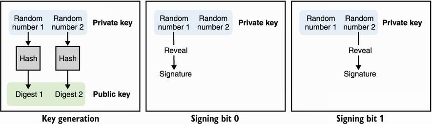
To sign a bit set to 0, reveal the x part of your private key; to sign a bit set to 1, reveal the y part. To verify a signature, simply hash it to check that it matches the correct part of the public key. I illustrate this in figure 14.1.
Figure 14.1 A Lamport signature is a one-time signature (OTS) based only on hash functions. To generate a key pair that can sign a bit, generate two random numbers, which will be your private key, and hash each of those individually to produce the two digests of your public key. To sign a bit set to 0, reveal the first random number; to sign a bit set to 1, reveal the second random number.
Signing a bit is not that useful, you say. No problem; a Lamport signature works for larger inputs simply by creating more pairs of secrets, one per bit, to sign (see figure 14.2). Obviously, if your input is larger than 256 bits, you would first hash it and then sign it.
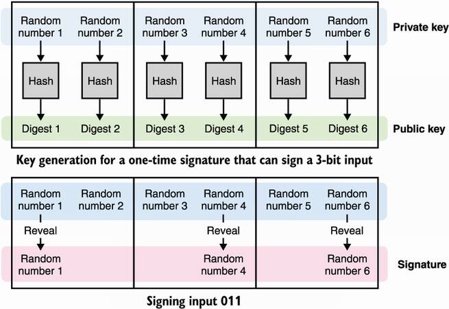
Figure 14.2 To generate a Lamport signature key pair that can sign an n-bit message, generate 2n random numbers, which will be your private key, and hash each of those individually to produce the 2n digests of your public key. To sign, go through pairs of secrets and n bits, revealing the first element to sign a bit set to 0 or the second element to sign a bit set to 1.
A major limitation of this scheme is that you can only use it to sign once; if you use it to sign twice, you end up authorizing someone else to mix the two signatures to forge other valid signatures. We can improve the situation naively by generating a large number of one-time key pairs instead of a single one, then making sure to discard a key pair after using it. Not only does this make your public key as big as the number of signatures you think you might end up using, but it also means you have to track what key pairs you’ve used (or better, get rid of the private keys you’ve used). For example, if you know you’ll want to sign a maximum of 1,000 messages of 256 bits with a hash function with a 256-bit output size, your private key and public key would both have to be 1000 × (256 × 2 × 256) bits, which is around 16 megabytes. That’s quite a lot for only 1,000 signatures.
Most of the hash-based signature schemes proposed today build on the foundations created by Lamport to allow for many more signatures (sometimes a practically unlimited amount of signatures), stateless private keys (although some proposed schemes are still stateful), and more practical parameter sizes.
A few months after Lamport’s publication, Robert Winternitz of the Stanford Mathematics Department proposed to publish hashes of hashes of a secret h(h(...h(x))) = hw(x) instead of publishing multiple digests of multiple secrets in order to optimize the size of a private key (see figure 14.3). This scheme is called Winternitz one-time signature (WOTS) after the author.
For example, choosing w = 16 allows you to sign 16 different values or, in other words, inputs of 4 bits. You start by generating a random value x that serves as your private key and hash that 16 times to obtain your public key, h16(x). Now imagine you want to sign the bits 1001 (9 in base 10); you publish the ninth iteration of the hash, h9(x). I illustrate this in figure 14.3.
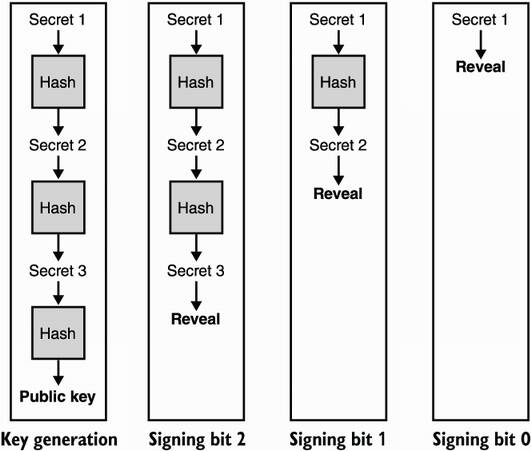
Figure 14.3 The Winternitz one-time signature (WOTS) scheme optimizes Lamport signatures by only using one secret that is hashed iteratively in order to obtain many other secrets and, finally, a public key. Revealing a different secret allows one to sign a different number.
Take a few minutes to understand how this scheme works. Do you see a problem with it? One major problem is that this scheme allows for signature forgeries. Imagine that you see someone else’s signature for bit 1001, which would be h9(x) according to our previous example. You can simply hash it to retrieve any other iterations like h10(x) or h11(x), which would give you a valid signature for bits 1010 or 1011. This can be circumvented by adding a short authentication tag after the message, which you would have to sign as well. I illustrate this in figure 14.4. To convince yourself that this solves the forgery issue, try to forge a signature from another signature.
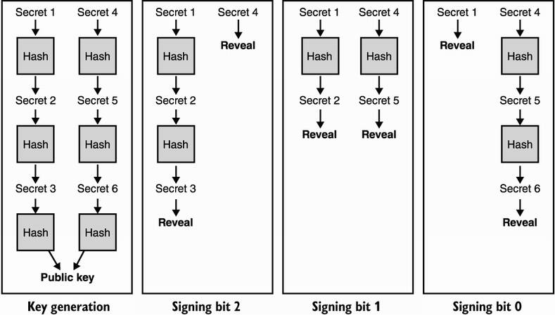
Figure 14.4 WOTS uses an additional signing key to authenticate a signature in order to prevent tampering. It works like this: when signing, the first private key is used to sign the message, and the second private key is used to sign the complement of the message. It should be clear that in any of the scenarios illustrated, tampering with a signature cannot lead to a new valid signature.
So far, you’ve seen ways of signing things using only hash functions. While Lamport signatures work, they have large key sizes, so WOTS improved on those by reducing the key sizes. Yet, both these schemes still don’t scale well as they are both one-time signatures (reuse a key pair and you break the scheme), and thus, their parameters linearly increase in size depending on the number of signatures you think you’ll need.
Some schemes that tolerate reuse of a key pair for a few signatures (instead of a single one) do exist. These schemes are called few-time signatures (FTS) and will break, allowing signature forgeries if reused too many times. FTS rely on low probabilities of reusing the same combination of secrets from a pool of secrets. This is a small improvement on one-time signatures, allowing a decrease in the risk of key reuse. But we can do better.
What is one technique you learned about in this book that compresses many things into one thing? The answer is Merkle trees. As you may recall from chapter 12, a Merkle tree is a data structure that provides short proofs for questions like is my data in this set? In the 1990s, the same Merkle who proposed Merkle trees also invented a signature scheme based on hash functions that compresses a number of one-time signatures into a Merkle tree.
The idea is pretty straightforward: each leaf of your tree is the hash of a one-time signature, and the root hash can be used as a public key, reducing its size to the output size of your hash function. To sign, you pick a one-time signature that you haven’t used previously and then apply it as explained in section 14.2.2. The signature is the one-time signature, along with the Merkle proof that it belongs in your Merkle tree (all the neighbors). This scheme is obviously stateful as one should be careful not to reuse one of the one-time signatures in the tree. I illustrate this in figure 14.5.
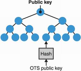
Figure 14.5 The Merkle signature scheme is a stateful hash-based algorithm that makes use of a Merkle tree to compress many OTS public keys into a smaller public key (the root hash). The larger the tree, the more signatures it can produce. Note that signatures now have the overhead of a membership proof, which is a number of neighbor nodes that allow one to verify that a signature’s associated OTS is part of the tree.
The extended Merkle signature scheme (XMSS), standardized in RFC 8391, sought to productionize Merkle signatures by adding a number of optimizations to Merkle’s scheme. For example, to produce a key pair capable of signing N messages, you must generate N OTS private keys. While the public key is now just a root hash, you still have to store N OTS private keys. XMSS reduces the size of the private key you hold by deterministically generating each OTS in the tree using a seed and the leaf position in the tree. This way, you only need to store the seed as a private key, instead of all the OTS private keys, and can quickly regenerate any OTS key pair from its position in the tree and the seed. To keep track of which leaf/OTS was used last, the private key also contains a counter that is incremented every time it is used to sign.
Having said that, there’s only so much OTS you can hold in a Merkle tree. The larger the tree, the longer it’ll take to regenerate the tree in order to sign messages (as you need to regenerate all the leaves to produce a Merkle proof). The smaller the tree, the fewer OTS private keys need to be regenerated when signing, but this obviously defeats the purpose: we are now back to having a limited amount of signatures. The solution is to use a smaller tree where the OTS in its leaves are not used to sign messages but, instead, used to sign the root hash of other Merkle trees of OTS. This transforms our initial tree into a hypertree—tree of trees—and is one of the variants of XMSS called XMSSMT. With XMSSMT, only the trees involved in the path of an OTS need to be regenerated, based on the same technique. I illustrate this in figure 14.6.
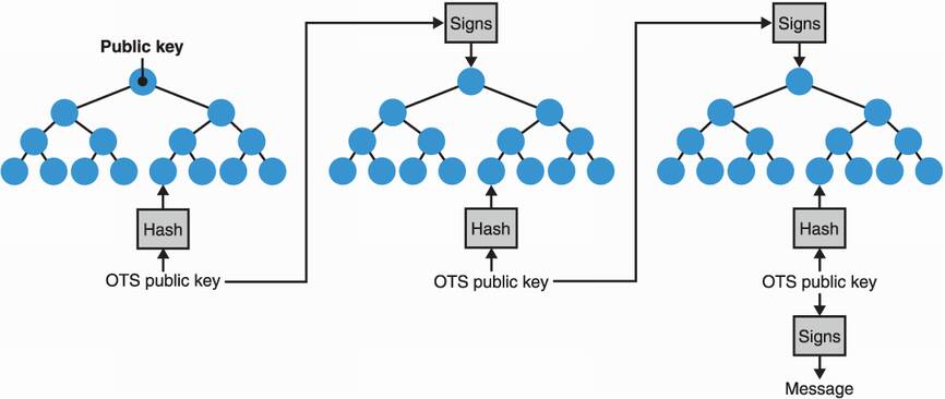
Figure 14.6 The XMSSMT stateful hash-based signature scheme uses multiple trees to increase the amount of signatures supported by the scheme while reducing the work at key generation and signing time. Each tree is deterministically generated only when they are used in the path to the final leaf that contains the OTS used to sign a message.
Note that the statefulness of XMSS and XMSSMT might not be an issue in some situations, but it is not a desirable property, in general. Having to keep track of a counter is counterintuitive as it is not expected from users of mainstream signature schemes. This change of practice can lead to OTS reuse (and, thus, to signature forgery) in case of misuse. For example, rollbacks to a previous state of the filesystem or using the same signing key on multiple servers might induce the same path in the hypertree being used twice to sign a message.
To fix one the biggest downsides of XMSS (its statefulness) and expose an interface similar to the signature schemes we’re used to, the SPHINCS+ signature scheme was proposed as part of the NIST’s post-quantum cryptography competition. The stateless signature scheme augments XMSSMT with three major changes:
Signing the same message twice leads to the same signature. In a similar fashion to EdDSA (covered in chapter 7), the path used in the hypertree is deterministically derived, based on the private key and the message. This ensures that signing the same message twice leads to the same OTS and, thus, the same signature; and because the private key is used, attackers are also unable to predict which path you’ll take to sign their messages if you somehow sign other people’s messages.
Using more trees. XMSSMT avoids reusing the same OTS twice by keeping track of which OTS was used last. As the whole point of SPHINCS+ is to avoid keeping track of a state, it needs to avoid collisions when it chooses a path pseudorandomly. To do this, SPHINCS+ simply uses a much larger amount of OTS, reducing the probability of reusing the same one twice. Because SPHINCS+ also uses a hypertree, this translates into more trees.
Using few-time signatures (FTS). As the security of the scheme is based on the probability of reusing the same path twice, SPHINCS+ also replaces the final OTS used to sign messages with the FTS I mentioned earlier. This way, reusing the same path to sign two different messages still doesn’t directly contribute to a break of the signature scheme.
While SPHINCS+ is being considered for standardization in the NIST post-quantum cryptography competition, it’s not the main contender. SPHINCS+ is not only slow, its signatures are large compared to the proposed alternatives (like lattice-based ones, which you’ll learn about later in this chapter). Stateful hash-based signature schemes like XMSS offer faster speed and better signature sizes (under 3 KB compared to the minimum of 8 KB for SPHINCS+). (In terms of public key sizes, both schemes provide sizes similar to pre-quantum signatures schemes like ECDSA and Ed25519.) Due to the more realistic parameter sizes and the well-understood security, XMSS is recommended as an early standard by the NIST in SP 800-208, “Recommendation for Stateful Hash-Based Signature Schemes.”
Next, let’s take a look at two other ways to build quantum-resistant cryptographic primitives. A gentle warning: they are much more math-heavy!
A large number of post-quantum cryptography schemes are based on lattices, a mathematical structure that you’ll learn about in this section. The NIST post-quantum cryptography competition itself has elected lattice-based schemes for half of its finalists. This makes lattice-based cryptography the most likely paradigm to win and obtain a standard from the NIST. In this section, I will tell you about two lattice-based algorithms: Dilithium, a signature scheme, and Kyber, a public key encryption primitive. But before that, though, let’s see what lattices are.
First, lattice-based probably doesn’t mean what you think it means. Take RSA (covered in chapter 6), which we say is based on the factorization problem. This does not mean that we use factorization in RSA, it instead means that factorization is how you attack RSA, and because factorization is hard, we say that RSA is secure. It’s the same with lattice-based cryptosystems: lattices are structures that have hard problems, and these cryptosystems are safe as long as these problems remain hard.
With that being said, what is a lattice? Well, it’s like a vector space but with integers. If you don’t remember what a vector space is, it’s the set of all vectors that can be created using:
An operation between vectors—The vectors can be added together; for example, (0,1) + (1,0) = (1,1).
A scalar operation—A vector can be multiplied by what we call scalars; for example, 3 × (1,2) = (3,6).
In our example, the vector space contains all the vectors that can be expressed as a linear combination of the basis, which translates to any vector that can be written as a × (0,1) + b × (1,0) for any scalars a and b. For example, 0.5 × (0,1) + 3.87 × (1,0) = (3.87,0.5) is in our vector space, so is 99 × (0,1) + 0 × (1,0) = (0,99), and so on.
A lattice is a vector space where all of the numbers involved are integers. Yup, in cryptography, we like integers. I illustrate this in figure 14.7.
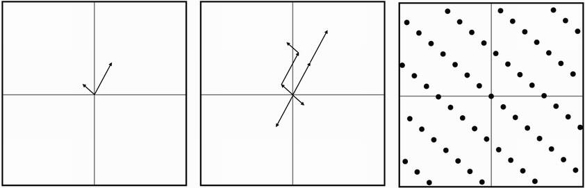
Figure 14.7 On the left, a basis of two vectors is drawn on a graph. A lattice can be formed by taking all of the possible integer linear combinations of these two vectors (middle figure). The resulting lattice can be interpreted as a pattern of points repeating forever in space (right figure).
There are several well-known hard problems in the lattice space, and for each of these problems, we have algorithms to solve them. These algorithms are often the best we could think of, but it doesn’t necessarily mean that they are efficient or even practical. Thus, the problems are said to be hard at least until an more efficient solution is found. The two most well-known hard problems are as follows. (I illustrate both of these problems in figure 14.8.)
The shortest vector problem (SVP)—Answers the question, what is the shortest nonzero vector in your lattice?
The closest vector problem (CVP)—Given a coordinate that is not on the lattice, finds the closest point to that coordinate on the lattice.
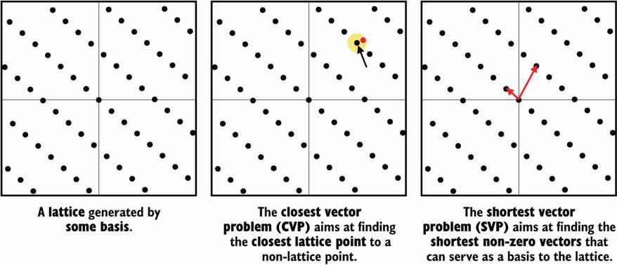
Figure 14.8 An illustration of the two major lattice problems used in cryptography: the shortest vector problem (SVP) and the closest vector problem (CVP)
Generally, we use algorithms like LLL (the Lenstra–Lenstra–Lovász algorithm) or BKZ (the Block-Korkine-Zolotarev algorithm) to solve both of these problems (CVP can be reduced to SVP). These are algorithms that reduce the basis of a lattice, meaning that they attempt to find a set of vectors that are shorter than the ones given and that managed to produce the exact same lattice.
In 2005, Oded Regev introduced the learning with errors (LWE) problem, which became the basis for many cryptographic schemes including some of the algorithms in this chapter. Before going further, let’s see what the LWE problem is about. Let’s start with the following equations, which are linear combinations of the same integers s0 and s1:
We know that by using the Gaussian elimination algorithm, we can quickly and efficiently learn what s0 and s1 are, as long as we have enough of these equations. Now what’s interesting is that if we add some noise to these equations, the problem becomes much harder:
While it probably isn’t too hard to figure out the answer given more noisy equations, it becomes a hard problem once you increase the size of the numbers involved and the number of si .
This is essentially what the LWE problem is, albeit often stated with vectors instead. Imagine that you have a secret vector s with coordinates modulo some large number. Given an arbitrary number of random vectors ai of the same size and the computations ais + ei , where ei is a random small error, can you find the value s?
Note For two vectors v and w, the product vw can be calculated using a dot product, which is the sum of the product of each pair of coordinates. Let’s look at an example: if v = (v0, v1) and w = (w0, w1), then vw = v0 × w0 + v1 × w1.
For example, if I use the secret s = (3,6) and I give you the random vectors a0 = (5,2) and a1 = (2,0), I get back the equations I started the example with. As I said earlier, lattice-based schemes actually don’t make any use of lattices; rather, they are proven secure if the SVP remains hard (for some definition of hard). The reduction can only be seen if we write the previous equations in a matrix form, as shown in figure 14.9.
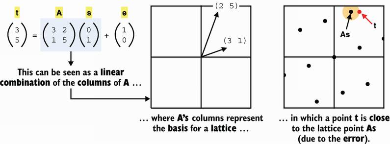
Figure 14.9 The learning with errors problem (LWE) is said to be a lattice-based construction due to the existence of a reduction to a lattice problem: the CVP. In other words, if we can find a solution to the CVP, then we can find a solution to the LWE problem.
This matrix form is important as most LWE-based schemes are expressed and easier to explain in this form. Take a few minutes to brush up on matrix multiplication. Also, in case you haven’t noticed, I used some common notational tricks that are quite helpful to read equations that involve matrices and vectors: both are written in bold, and matrices are always uppercase letters. For example, A is a matrix, a is a vector, and b is just a number.
Note There exist several variants of the LWE problem (for example, the ring-LWE or module-LWE problems), which are basically the same problem but with coordinates in different types of groups. These variants are often preferred due to the compactness and the optimizations they unlock. The difference between the variants of LWE does not affect the explanations that follow.
Now that you know what the LWE problem is, let’s learn about some post-quantum cryptography based on it: the Cryptographic Suite for Algebraic Lattices (CRYSTALS). Conveniently, CRYSTALS encompasses two cryptographic primitives: a key exchange called Kyber and a signature scheme called Dilithium.
Two NIST finalist schemes are closely related: CRYSTALS-Kyber and CRYSTALS-Dilithium, which are candidates from the same team of researchers and are both based on the LWE problem. Kyber is a public key encryption primitive that can be used as a key exchange primitive, which I will explain in this section. Dilithium is a signature scheme, which I will explain in the next section. Also note that as these algorithms are still in flux, I will only write about the ideas and the intuitions behind both of the schemes.
First, let’s assume that all operations happen in a group of integers modulo a large number q. Let’s also say that errors and private keys are sampled (chosen uniformly at random) from a small range centered at 0 that we will call the error range. Specifically, the error range is the range [–B, B] where B is much smaller than q. This is important as some terms need to be smaller than some value to be considered errors.
To generate the private key, simply generate a random vector s, where every coefficient is in the error range. The first part of the public key is a list of random vectors ai of the same size, and the second part is the associated list of noisy dot products ti = ai s + ei mod q. This is exactly the LWE problem we learned about previously. Importantly for the rest, we can rewrite this with matrices:
where the matrix A contains the random vectors ai as rows, and the error vector e contains the individual errors ei .
To perform a key exchange with Kyber, we encrypt a symmetric key of 1 bit (yes, a single bit!) with the scheme. This is akin to the RSA key encapsulation mechanism you saw in chapter 6. The following four steps shows how the encryption works:
Generate an ephemeral private key vector r (where coefficients are in the error range) and its associated ephemeral public key rA + e1 with some random error vector e1, using the other peer’s A matrix as a public parameter. Note that the matrix multiplication is done on the right, which involves multiplying the vector r with the columns of A instead of computing Ar (a multiplication of the vector r with the rows of A). It is a detail, but it’s necessary for the decryption step to work.
We shift our message to the left by multiplying it with q/2 in order to avoid small errors from impacting our message. Note that q/2 modulo q usually means q multiplied with the inverse of 2 modulo q, but here it simply means the closest integer to q/2.
Compute a shared secret with the dot product of our ephemeral private key and the public key of the peer.
Encrypt your (shifted) message by adding it to the shared secret as well as a random error e2. This produces a ciphertext.
After performing the steps, we can send both the ephemeral public key and the ciphertext to the other peer. After receiving both the ephemeral public key and the ciphertext, we can follow these steps to decrypt the message:
Obtain the shared secret by computing the dot product of your secret with the ephemeral public key received.
Subtract that shared secret from the ciphertext (the result contains the shifted message and some error).
Shift your message back to where it was originally by dividing it with q/2, effectively removing the error.
The message is 1 if it is closer to q/2 than 0, and it is 0 otherwise.
Of course, 1 bit is not enough, so current schemes employ different techniques to overcome this limitation. I recapitulate all three algorithms in figure 14.10.
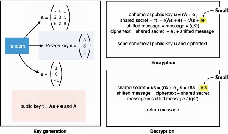
Figure 14.10 The Kyber public key encryption scheme. Note that the shared secret is approximately the same during encryption and decryption as re and e1s are both small values because r, s, and the errors are much smaller than q/2). Thus, the last step of the decryption (dividing by q/2, which can be seen as a bitwise shift to the right) gets rid of any discrepancy between the two shared secrets. Note that all operations are done modulo q.
In practice, for a key exchange, the message you encrypt to your peer’s public key is a random secret. The result is then derived deterministically from both the secret and the transcript of the key exchange, which includes the peer’s public key, your ephemeral key, and the ciphertext.
The recommended parameters for Kyber leads to public keys and ciphertexts of around 1 kilobytes, which is much bigger than the pre-quantum schemes we use but still in the realm of the practical for most use cases. While time will tell if we can further reduce the communication overhead of these schemes, it seems like, so far, post-quantum rhymes with larger sizes.
The next scheme I’ll explain, Dilithium, is also based on LWE and is the sister candidate of Kyber. As with other types of signatures we’ve seen (like Schnorr’s signature in chapter 7), Dilithium is based on a zero-knowledge proof that is made non-interactive via the Fiat-Shamir trick.
For key generation, Dilithium is similar to the previous scheme, except that we keep the error as part of the private key. We first generate the two random vectors that serve as the private key, s1 and s2, then compute the public key as t = As1 + s2, where A is a matrix obtained in a similar manner as Kyber. The public key is t and A. Note that we consider the error s2 as being part of the private key because we need to reuse it every time we sign a message (unlike in Kyber, where the error could be discarded after the key generation step).
To sign, we create a sigma protocol and then convert that to a non-interactive, zero-knowledge proof via the Fiat-Shamir transformation, which is similar to how the Schnorr identification protocol gets converted to a Schnorr signature in chapter 7. The interactive protocol looks like this:
The prover commits on two random vectors, y1 and y2, by sending Ay1 + y2.
Upon reception of this commit, the verifier responds with a random challenge c.
The prover then computes the two vectors z1 = c s1 + y1 and z2 = c s2 + y2 and sends them to the verifier only if they are small values.
The verifier checks if Az1 + z2 – c t and Ay1 + y2 are the same values.
The Fiat-Shamir trick replaces the role of the verifier in step 2 by having the prover generate a challenge from a hash of the message to sign and the committed Ay1 + y2 value. I recap this transformation in figure 14.11, using a similar diagram from chapter 7.
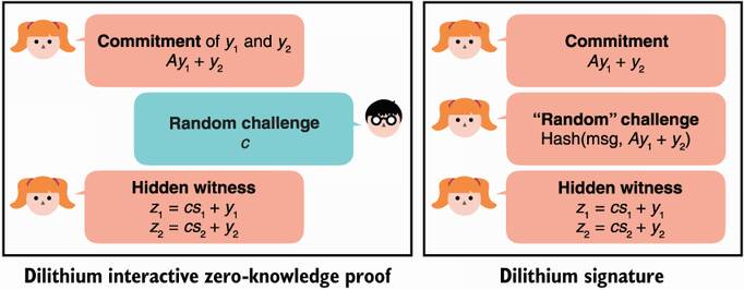
Figure 14.11 A Dilithium signature is a proof of knowledge of a secret vector s made non-interactive via the Fiat-Shamir transformation. The diagram on the left shows the interactive proof protocol, while the diagram on the right shows a non-interactive version where the challenge is computed as a commitment of both y and the message to sign.
Again, this is a gross simplification of the signature scheme. Many more optimizations are used in practice to reduce the key and the signature sizes. Usually, these optimizations look at reducing any random data by deterministically generating it from a smaller random value and by reducing non-random data by compressing it via custom methods, not necessarily via known compression algorithms. There are also a number of additional optimizations that are possible due to the unique structure of LWE.
At the recommended security level, Dilithium offers signatures of around 3 KB and public keys of less than 2 KB. This is obviously much more than the 32-byte public keys and 64-byte signatures of pre-quantum schemes, but it is also much better than the stateless hash-based signatures. It is good to keep in mind that these schemes are still pretty new, and it is possible that better algorithms will be found to solve the LWE problem, potentially increasing the sizes of public keys and signatures. It is also possible that we will find better techniques to reduce the sizes of these parameters. In general, it’s likely that quantum resistance will always come with a cost in size.
This is not all there is to post-quantum cryptography; the NIST post-quantum cryptography competition has a number of other constructions based on different paradigms. NIST has announced that an initial standard will be published in 2022, but I expect that the field will continue to move quickly, at least as long as post-quantum computers continue to be seen as a legitimate threat. While there’s still a lot of unknowns, it also means that there’s a lot of exciting room for research. If this is interesting to you, I recommend taking a look at the NIST reports (https://nist.gov/pqcrypto).
To summarize, quantum computers are a huge deal for cryptography if they are realized. What’s the take away here? Do you need to throw everything you’re doing and transition to post-quantum algorithms? Well, it’s not that simple.
Ask any expert and you’ll receive different kinds of answers. For some, it’s 5 to 50 years away; for others, it’ll never happen. Michele Mosca, the director of the Institute for Quantum Computing, estimated “a 1/7 chance of breaking RSA-2048 by 2026 and a 1/2 chance by 2031,” while Mikhail Dyakonov, a researcher at the CNRS in France, stated publicly “Could we ever learn to control the more than 10300 continuously variable parameters defining the quantum state of such a system? My answer is simple. No, never.” While physicists, not cryptographers, know better, they can still be incentivized to hype their own research in order to get funding. As I am no physicist, I will simply say that we should remain skeptical of extraordinary claims, while preparing for the worst. The question is not “Will it work?”; rather, it’s “Will it scale?”
There exist many challenges for scalable quantum computers (which can destroy cryptography) to become a reality; the biggest ones seem to be about the amount of noise and errors that is difficult to reduce or correct. Scott Aaronson, a computer scientist at the University of Texas, puts it as “You’re trying to build a ship that remains the same ship, even as every plank in it rots and has to be replaced.”
But what about what the NSA said? One needs to remember that the government’s need for confidentiality most often exceeds the needs of individuals and private companies. It is not crazy to think that the government might want to keep some top secret data classified for more than 50 years. Nevertheless, this has puzzled many cryptographers (see, for example, “A Riddle Wrapped In An Enigma” by Neal Koblitz and Alfred J. Menezes), who have been wondering why we would protect ourselves against something that doesn’t exist yet or might never exist.
In any case, if you’re really worried and the confidentiality of your assets needs to remain for long periods of time, it is not crazy and relatively easy to increase the parameters of every symmetric cryptographic algorithm you’re using. That being said, if you’re doing a key exchange in order to obtain an AES-256-GCM key, that asymmetric cryptography part is still vulnerable to quantum computers, and protecting the symmetric cryptography alone won’t be enough.
For asymmetric cryptography, it is too early to really know what is safe to use. Best wait for the end of the NIST competition in order to obtain more cryptanalysis, and in turn, more confidence in these novel algorithms.
At present, there are several post-quantum cryptosystems that have been proposed, including lattice-based cryptosystems, code-based cryptosystems, multivariate cryptosystems, hash-based signatures, and others. However, for most of these proposals, further research is needed in order to gain more confidence in their security (particularly against adversaries with quantum computers) and to improve their performance.
—NIST Post-Quantum Cryptography Call for Proposals (2017)
If you’re too impatient and can’t wait for the result of the NIST competition, one thing you can do is to use both a current scheme and a post-quantum scheme in your protocol. For example, you could cross-sign messages using Ed25519 and Dilithium or, in other words, attach a message with two signatures from two different signature schemes. If it turns out that Dilithium is broken, an attacker would still have to break Ed25519, and if it turns out that quantum computers are real, then the attacker would still have the Dilithium signature that they can’t forge.
Note This is what Google did in 2018, and then again in 2019, with Cloudflare, experimenting with a hybrid key exchange scheme in TLS connections between a small percentage of Google Chrome users and servers from both Google and Cloudflare. The hybrid scheme was a mix of X25519 and one post-quantum key exchange (New Hope in 2018, HRSS and SIKE in 2019), where both the output of the current key exchange and the post-quantum key exchange were mixed together into HKDF to produce a single shared secret.
Finally, I will re-emphasize that hash-based signatures are well studied and well understood. Even though they present some overhead, schemes like XMSS and SPHINCS+ can be used now, and XMSS has ready-to-use standards (RFC 8391 and NIST SP 800-208).
Quantum computers are based on quantum physics and can provide a non-negligible speed up for specific computations.
Not all algorithms can run on a quantum computer, and not all algorithms can compete with a classical computer. Two notable algorithms that worry cryptographers are
The field of post-quantum cryptography aims at finding novel cryptographic algorithms to replace today’s asymmetric cryptographic primitives (for example, asymmetric encryption, key exchanges, and digital signatures).
NIST started a post-quantum cryptography standardization effort in 2016. There are currently seven finalists and the effort is now entering its final round of selection.
Hash-based signatures are signature schemes that are only based on hash functions. The two main standards are XMSS (a stateful signature scheme) and SPHINCS+ (a stateless signature scheme).
Lattice-based cryptography is promising as it provides shorter keys and signatures. Two of the most promising candidates are based on the LWE problem: Kyber is an asymmetric encryption and key exchange primitive, and Dilithium is a signature scheme.
Other post-quantum schemes exist and are being proposed as part of the NIST post-quantum cryptography competition. These include schemes based on code theory, isogenies, symmetric-key cryptography, and multivariate polynomials. NIST’s competition is scheduled to end in 2022, which still leaves a lot of room for new attacks or optimizations to be discovered.
It is not clear when quantum computers will be efficient enough to destroy cryptography, or if it is possible for them to get there.
If you have requirements to protect data for a long period of time, you should consider transitioning to post-quantum cryptography: