You’re about to learn one of the most ubiquitous and powerful cryptographic primitives—digital signatures. To put it simply, digital signatures are similar to the real-life signatures that you’re used to, the ones that you scribe on checks and contracts. Except, of course, that digital signatures are cryptographic and so they provide much more assurance than their pen-and-paper equivalents.
In the world of protocols, digital signatures unlock so many different possibilities that you’ll run into them again and again in the second part of this book. In this chapter, I will introduce what this new primitive is, how it can be used in the real world, and what the modern digital signature standards are. Finally, I will talk about security considerations and the hazards of using digital signatures.
Note Signatures in cryptography are often referred to as digital signatures or signature schemes. In this book, I interchangeably use these terms.
For this chapter, you’ll need to have read
I explained in chapter 1 that cryptographic signatures are pretty much like real-life signatures. For this reason, they are usually one of the most intuitive cryptographic primitives to understand:
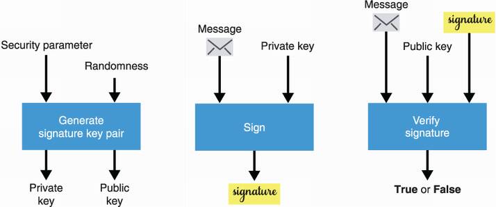
As we’re in the realm of asymmetric cryptography, you can probably guess how this asymmetry is going to take place. A signature scheme typically consists of three different algorithms:
A key pair generation algorithm that a signer uses to create a new private and public key (the public key can then be shared with anyone).
A signing algorithm that takes a private key and a message to produce a signature.
A verifying algorithm that takes a public key, a message, and a signature and returns a success or error message.
Sometimes the private key is also called the signing key, and the public key is called the verifying key. Makes sense, right? I recapitulate these three algorithms in figure 7.1.
Figure 7.1 The interface of a digital signature. Like other public key cryptographic algorithms, you first need to generate a key pair via a key generation algorithm that takes a security parameter and some randomness. You can then use a signing algorithm with the private key to sign a message and a verifying algorithm with the public key to validate a signature over a message. You can’t forge a signature that verifies a public key if you don’t have access to its associated private key.
What are signatures good for? They are good for authenticating the origin of a message as well as the integrity of a message:
Note While these two properties are linked to authentication, they are often distinguished as two separate properties: origin authentication and message authentication (or integrity).
In a sense, signatures are similar to the message authentication codes (MACs) that you learned about in chapter 3. But unlike MACs, they allow us to authenticate messages asymmetrically: a participant can verify that a message hasn’t been tampered without knowledge of the private or signing key. Next, I’ll show you how these algorithms can be used in practice.
Let’s look at a practical example. For this, I use pyca/cryptography (https://cryptography.io), a well-respected Python library. The following listing simply generates a key pair, signs a message using the private key part, and then verifies the signature using the public key part.
Listing 7.1 Signing and verifying signatures in Python
from cryptography.hazmat.primitives.asymmetric.ed25519 import (
    Ed25519PrivateKey                                              ❶
)

private_key = Ed25519PrivateKey.generate()                         ❷
public_key = private_key.public_key()                              ❷

message = b"example.com has the public key 0xab70..."              ❸
signature = private_key.sign(message)                              ❸

try:                                                               ❹
    public_key.verify(signature, message)                          ❹
    print("valid signature")                                       ❹
except InvalidSignature:                                           ❹
    print("invalid signature")                                     ❹
❶ Uses the Ed25519 signing algorithm, a popular signature scheme
❷ First generates the private key and then generates the public key
❸ Using the private key, signs a message and obtains a signature
❹ Using the public key, verifies the signature over the message
As I said earlier, digital signatures unlock many use cases in the real world. Let’s see an example in the next section.
Chapters 5 and 6 introduced different ways to perform key exchanges between two participants. In the same chapters, you learned that these key exchanges are useful to negotiate a shared secret, which can then be used to secure communications with an authenticated encryption algorithm. Yet, key exchanges didn’t fully solve the problem of setting up a secure connection between two participants as an active man-in-the-middle (MITM) attacker can trivially impersonate both sides of a key exchange. This is where signatures enter the ring.
Imagine that Alice and Bob are trying to set up a secure communication channel between themselves and that Bob is aware of Alice’s verifying key. Knowing this, Alice can use her signing key to authenticate her side of the key exchange: she generates a key exchange key pair, signs the public key part with her signing key, then sends the key exchange public key along with the signature. Bob can verify that the signature is valid using the associated verifying key he already knows and then use the key exchange public key to perform a key exchange.
We call such a key exchange an authenticated key exchange. If the signature is invalid, Bob can tell someone is actively MITM’ing the key exchange. I illustrate authenticated key exchanges in figure 7.2.
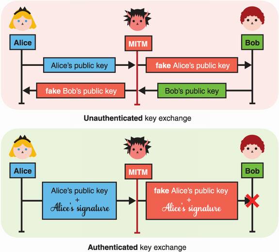
Figure 7.2 The first picture (top) represents an unauthenticated key exchange, which is insecure to an active MITM attacker who can trivially impersonate both sides of the exchange by swapping their public keys with their own. The second picture (bottom) represents the beginning of a key exchange, authenticated by Alice’s signature over her public key. As Bob (who knows Alice’s verifying key) is unable to verify the signature after the message was tampered by the MITM attacker, he aborts the key exchange.
Note that in this example, the key exchange is only authenticated on one side: while Alice cannot be impersonated, Bob can. If both sides are authenticated (Bob would sign his part of the key exchange), we call the key exchange a mutually-authenticated key exchange. Signing key exchanges might not appear super useful yet. It seems like we moved the problem of not knowing Alice’s key exchange public key in advance to the problem of not knowing her verifying key in advance. The next section introduces a real-world use of authenticated key exchanges that will make much more sense.
Signatures become much more powerful if you assume that trust is transitive. By that, I mean that if you trust me and I trust Alice, then you can trust Alice. She’s cool.
Transitivity of trust allows you to scale trust in systems in extreme ways. Imagine that you have confidence in some authority and their verifying key. Furthermore, imagine that this authority has signed messages indicating what the public key of Charles is, what the public key of David is, and so on. Then, you can choose to have faith in this mapping! Such a mapping is called a public key infrastructure. For example, if you attempt to do a key exchange with Charles and he claims that his public key is a large number that looks like 3848 . . . , you can verify that by checking if your “beloved” authority has signed some message that looks like “the public key of Charles is 3848 . . .”
One real-world application of this concept is the web public key infrastructure (web PKI). The web PKI is what your web browser uses to authenticate key exchanges it performs with the multitude of websites you visit every day. A simplified explanation of the web PKI (illustrated in figure 7.3) is as follows: when you download a browser, it comes with some verifying key baked into the program. This verifying key is linked to an authority whose responsibility is to sign thousands and thousands of websites’ public keys so that you can trust these without knowing about them. What you’re not seeing is that these websites have to prove to the authority that they truly own their domain name before they can obtain a signature on their public key. (In reality, your browser trusts many authorities to do this job, not just a single one.)
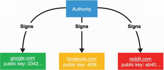
Figure 7.3 In the web PKI, browsers trust an authority to certify that some domains are linked to some public keys. When visiting a website securely, your browser can verify that the website’s public key is indeed theirs (and not from some MITM) by verifying a signature from the authority.
In this section, you learned about signatures from a high-level point of view. Let’s dig deeper into how signatures really work. But for this, we first need to make a detour and take a look at something called a zero-knowledge proof (ZKP).
The best way to understand how signatures work in cryptography is to understand where they come from. For this reason, let’s take a moment to briefly introduce ZKPs and then I’ll get back to signatures.
Imagine that Peggy wants to prove something to Victor. For example, she wants to prove that she knows the discrete logarithm to the base of some group element. In other words, she wants to prove that she knows x given Y = gx with g the generator of some group.
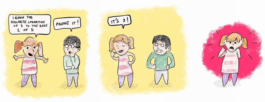
Of course, the simplest solution is for Peggy to simply send the value x (called the witness). This solution would be a simple proof of knowledge, and this would be OK, unless Peggy does not want Victor to learn it.
Note In theoretical terms, we say that the protocol to produce a proof is complete if Peggy can use it to prove to Victor that she knows the witness. If she can’t use it to prove what she knows, then the scheme is useless, right?
In cryptography, we’re mostly interested in proofs of knowledge that don’t divulge the witness to the verifier. Such proofs are called zero-knowledge proofs (ZKPs).
In the next pages, I will build a ZKP incrementally from broken protocols to show you how Alice can prove that she knows x without revealing x.
The typical way to approach this kind of problem in cryptography is to “hide” the value with some randomness (for example, by encrypting it). But we’re doing more than just hiding: we also want to prove that it is there. To do that, we need an algebraic way to hide it. A simple solution is to simply add a randomly generated value k to the witness:
Peggy can then send the hidden witness s along with the random value k to Victor. At this point, Victor has no reason to trust that Peggy did, in fact, hide the witness in s. Indeed, if she doesn’t know the witness x then s is probably just some random value. What Victor does know is that the witness x is hiding in the exponent of g because he knows Y = gx.
To see if Peggy really knows the witness, Victor can check if what she gave him matches what he knows, and this has to be done in the exponent of g as well (as this is where the witness is). In other words, Victor checks that these two numbers are equal:
The idea is that only someone who knows the witness x could have constructed a “blinded” witness s that satisfies this equation. And as such, it’s a proof of knowledge. I recapitulate this ZKP system in figure 7.4.
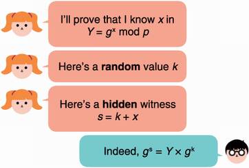
Figure 7.4 In order to prove to Victor that she knows a witness x, Peggy hides it (by adding it to a random value k) and sends the hidden witness s instead.
Not so fast. There’s one problem with this scheme—it’s obviously not secure! Indeed, because the equation hiding the witness x only has one unknown (x itself), Victor can simply reverse the equation to retrieve the witness:
To fix this, Peggy can hide the random value k itself! This time, she has to hide the random value in the exponent (instead of adding it to another random value) to make sure that Victor’s equation still works:
This way, Victor does not learn the value k (this is the discrete logarithm problem covered in chapter 5) and, thus, cannot recover the witness x. Yet, he still has enough information to verify that Peggy knows x! Victor simply has to check that gs (= gk+x = gk × gx) is equal to Y × R (= gx × gk). I review this second attempt at a ZKP protocol in figure 7.5.
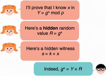
Figure 7.5 To make a knowledge proof zero-knowledge, the prover can hide the witness x with a random value k and then hide the random value itself.
There is one last issue with our scheme—Peggy can cheat. She can convince Victor that she knows x without knowing x! All she has to do is to reverse the step in which she computes her proof. She first generates a random value s and then calculates the value R based on s:
Victor then computes Y × R = Y × gs × Y–1, which indeed matches gs. (Peggy’s trick of using an inverse to compute a value is used in many attacks in cryptography.)
Note In theoretical terms, we say that the scheme is “sound” if Peggy cannot cheat (if she doesn’t know x, then she can’t fool Victor).
To make the ZKP protocol sound, Victor must ensure that Peggy computes s from R and not the inverse. To do this, Victor makes the protocol interactive:
Peggy must commit to her random value k so that she cannot change it later.
After receiving Peggy’s commitment, Victor introduces some of his own randomness in the protocol. He generates a random value c (called a challenge) and sends it to Peggy.
Peggy can then compute her hidden commit based on the random value k and the challenge c.
Note You learned about commitment schemes in chapter 2 where we used a hash function to commit to a value that we can later reveal. But commitment schemes based on hash functions do not allow us to do interesting arithmetic on the hidden value. Instead, we can simply raise our generator to the value, gk, which we’re already doing.
Because Peggy cannot perform the last step without Victor’s challenge c, and Victor won’t send that to her without seeing a commitment on the random value k, Peggy is forced to compute s based on k. The obtained protocol, which I illustrate in figure 7.6, is often referred to as the Schnorr identification protocol.
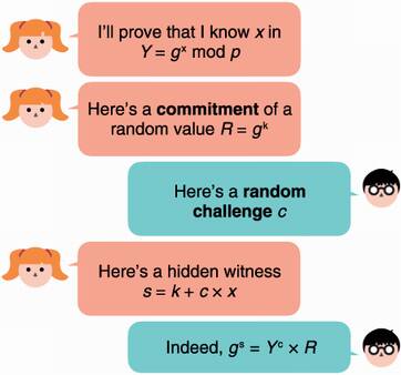
Figure 7.6 The Schnorr identification protocol is an interactive ZKP that is complete (Peggy can prove she knows some witness), sound (Peggy cannot prove anything if she doesn’t know the witness), and zero-knowledge (Victor learns nothing about the witness).
So-called interactive ZKP systems that follow a three-movement pattern (commitment, challenge, and proof) are often referred to as Sigma protocols in the literature and are sometimes written as Σ protocols (due to the illustrative shape of the Greek letter). But what does that have to do with digital signatures?
Note The Schnorr identification protocol works in the honest verifier zero-knowledge (HVZK) model : if the verifier (Victor) acts dishonestly and does not choose a challenge randomly, they can learn something about the witness. Some stronger ZKP schemes are zero-knowledge even when the verifier is malicious.
The problem with the previous interactive ZKP is that, well, it’s interactive, and real-world protocols are, in general, not fond of interactivity. Interactive protocols add some non-negligible overhead as they require several messages (potentially over the network) and add unbounded delays, unless the two participants are online at the same time. Due to this, interactive ZKPs are mostly absent from the world of applied cryptography.
All of this discussion is not for nothing though! In 1986, Amos Fiat and Adi Shamir published a technique that allowed one to easily convert an interactive ZKP into a non-interactive ZKP. The trick they introduced (referred to as the Fiat-Shamir heuristic or Fiat-Shamir transformation) was to make the prover compute the challenge themselves, in a way they can’t control.
Here’s the trick—compute the challenge as a hash of all the messages sent and received as part of the protocol up to that point (which we call the transcript). If we assume that the hash function gives outputs that are indistinguishable from truly-random numbers (in other words, it looks random), then it can successfully simulate the role of the verifier.
Schnorr went a step further. He noticed that anything can be included in that hash! For example, what if we included a message in there? What we obtain is not only a proof that we know some witness x, but a commitment to a message that is cryptographically linked to the proof. In other words, if the proof is correct, then only someone with the knowledge of the witness (which becomes the signing key) could have committed that message.
That’s a signature! Digital signatures are just non-interactive ZKPs. Applying the Fiat-Shamir transform to the Schnorr identification protocol, we obtain the Schnorr signature scheme, which I illustrate in figure 7.7.
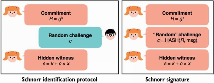
Figure 7.7 The left protocol is the Schnorr identification protocol previously discussed, which is an interactive protocol. The right protocol is a Schnorr signature, which is a non-interactive version of the left protocol (where the verifier message is replaced by a call to a hash function on the transcript).
To recapitulate, a Schnorr signature is essentially two values, R and s, where R is a commitment to some secret random value (which is often called a nonce as it needs to be unique per signature), and s is a value computed with the help of the commitment R, the private key (the witness x), and a message. Next, let’s look at the modern standards for signature algorithms.
Like other fields in cryptography, digital signatures have many standards, and it is sometimes hard to understand which one to use. This is why I’m here! Fortunately, the types of algorithms for signatures are similar to the ones for key exchanges: there are algorithms based on arithmetic modulo a large number like Diffie-Hellman (DH) and RSA, and there are algorithms based on elliptic curves like Elliptic Curve Diffie-Hellman (ECDH).
Be sure you understand the algorithms in chapter 5 and chapter 6 well enough as we’re now going to build on those. Interestingly, the paper that introduced the DH key exchange also proposed the concept of digital signatures (without giving a solution):
In order to develop a system capable of replacing the current written contract with some purely electronic form of communication, we must discover a digital phenomenon with the same properties as a written signature. It must be easy for anyone to recognize the signature as authentic, but impossible for anyone other than the legitimate signer to produce it. We will call any such technique one-way authentication. Since any digital signal can be copied precisely, a true digital signature must be recognizable without being known.
—Diffie and Hellman (“New Directions in Cryptography,” 1976)
A year later (in 1977), the first signature algorithm (called RSA) was introduced along with the RSA asymmetric encryption algorithm (which you learned about in chapter 6). RSA for signing is the first algorithm we’ll learn about.
In 1991, NIST proposed the Digital Signature Algorithm (DSA) as an attempt to avoid the patents on Schnorr signatures. For this reason, DSA is a weird variant of Schnorr signatures, published without a proof of security (although no attacks have been found so far). The algorithm was adopted by many but was quickly replaced with an elliptic curve version called ECDSA (for Elliptic Curve Digital Signature Algorithm), the same way Elliptic Curve Diffie-Hellman (ECDH) replaced Diffie-Hellman (DH), thanks to its smaller keys (see chapter 5). ECDSA is the second signature algorithm I will talk about in this section.
After the patents on Schnorr signatures expired in 2008, Daniel J. Bernstein, the inventor of ChaCha20-Poly1305 (covered in chapter 4) and X25519 (covered in chapter 5), introduced a new signature scheme called EdDSA (for Edwards-curve Digital Signature Algorithm), based on Schnorr signatures. Since its invention, EdDSA has quickly gained adoption and is nowadays considered state-of-the-art in terms of a digital signature for real-world applications. EdDSA is the third and last signature algorithm I will talk about in this section.
RSA signatures are currently used everywhere, even though they shouldn’t be (as you will see in this section, they present many issues). This is due to the algorithm being the first signature scheme to be standardized as well as real-world applications being slow to move to newer and better algorithms. Because of this, you will most likely encounter RSA signatures in your journey, and I cannot avoid explaining how they work and which standards are the adopted ones. But let me say that if you understood how RSA encryption works in chapter 6, then this section should be straightforward because signing with RSA is the opposite of encrypting with RSA:
To sign, you encrypt the message with the private key (instead of the public key), which produces a signature (a random element in the group).
To verify a signature, you decrypt the signature with the public key (instead of the private key). If it gives you back the original message, then the signature is valid.
Note In reality, a message is often hashed before being signed as it’ll take less space (RSA can only sign messages that are smaller than its modulus). The result is also interpreted as a large number so that it can be used in mathematical operations.
If your private key is the private exponent d, and your public key is the public exponent e and public modulus N, you can
I illustrate this visually in figure 7.8.
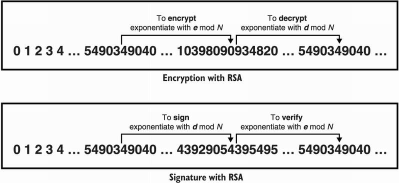
Figure 7.8 To sign with RSA, we simply do the inverse of the RSA encryption algorithm: we exponentiate the message with the private exponent, then to verify, we exponentiate the signature with the public exponent, which returns to the message.
This works because only the one knowing about the private exponent d can produce a signature over a message. And, as with RSA encryption, the security is tightly linked with the hardness of the factorization problem.
What about the standards to use RSA for signatures? Luckily, they follow the same pattern as does RSA encryption:
RSA for encryption was loosely standardized in the PKCS#1 v1.5 document. The same document contained a specification for signing with RSA (without a security proof).
RSA was then standardized again in the PKCS#1 v2 document with a better construction (called RSA-OAEP). The same happened for RSA signatures with RSA-PSS being standardized in the same document (with a security proof).
I talked about RSA PKCS#1 v1.5 in chapter 6 on asymmetric encryption. The signature scheme standardized in that document is pretty much the same as the encryption scheme. To sign, first hash the message with a hash function of your choice, then pad it according to PKCS#1 v1.5’s padding for signatures (which is similar to the padding for encryption in the same standard). Next, encrypt the padded and hashed message with your private exponent. I illustrate this in figure 7.9.
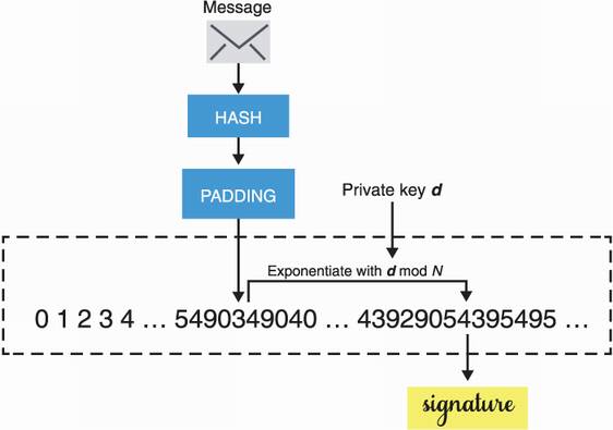
Figure 7.9 RSA PKCS#1 v1.5 for signatures. To sign, hash then pad the message with the PKCS#1 v1.5 padding scheme. The final step exponentiates the padded hashed message with the private key d modulo N. To verify, simply exponentiate the signature with the public exponent e modulo N and verify that it matches the padded and hashed message.
In chapter 6, I mentioned that there were damaging attacks on RSA PKCS#1 v1.5 for encryption; the same is unfortunately true for RSA PKCS#1 v1.5 signatures. In 1998, after Bleichenbacher found a devastating attack on RSA PKCS#1 v1.5 for encryption, he decided to take a look at the signature standard. Bleichenbacher came back in 2006 with a signature forgery attack on RSA PKCS#1 v1.5, one of the most catastrophic types of attack on signatures—attackers can forge signatures without knowledge of the private key! Unlike the first attack that broke the encryption algorithm directly, the second attack was an implementation attack. This meant that if the signature scheme was implemented correctly (according to the specification), the attack did not work.
An implementation flaw doesn’t sound as bad as an algorithm flaw, that is, if it’s easy to avoid and doesn’t impact many implementations. Unfortunately, it was shown in 2019 that an embarrassing number of open source implementations of RSA PKCS#1 v1.5 for signatures actually fell for that trap and misimplemented the standard (see “Analyzing Semantic Correctness with Symbolic Execution: A Case Study on PKCS#1 v1.5 Signature Verification” by Chau et al.) The various implementation flaws ended up enabling different variants of Bleichenbacher’s forgery attack.
Unfortunately, RSA PKCS#1 v1.5 for signatures is still widely used. Be aware of these issues if you really have to use this algorithm for backward compatibility reasons. Having said that, this does not mean that RSA for signatures is insecure. The story does not end here.
RSA-PSS was standardized in the updated PKCS#1 v2.1 and included a proof of security (unlike the signature scheme standardized in the previous PKCS#1 v1.5). The newer specification works like this:
The PSS encoding is a bit more involved and similar to OAEP (Optimal Asymmetric Encryption Padding). I illustrate this in figure 7.10.
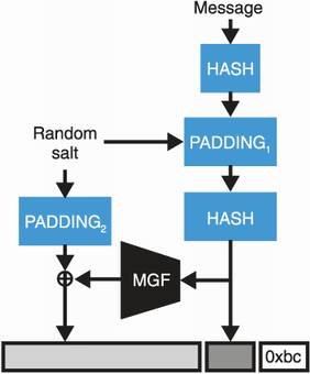
Figure 7.10 The RSA-PSS signature scheme encodes a message using a mask generation function (MGF) like the RSA-OAEP algorithm you learned about in chapter 6 before signing it in the usual RSA way.
Verifying a signature produced by RSA-PSS is just a matter of inverting the encoding once the signature has been raised to the public exponent modulo the public modulus.
If you remember, I also talked about a third algorithm in chapter 6 for RSA encryption (called RSA-KEM)—a simpler algorithm that is not used by anyone and yet is proven to be secure as well. Interestingly, RSA for signatures also mirror this part of the RSA encryption history and has a much simpler algorithm that pretty much nobody uses; it’s called Full Domain Hash (FDH). FDH works by simply hashing a message and then signing it (by interpreting the digest as a number) using RSA.
Despite the fact that both RSA-PSS and FDH come with proofs of security and are much easier to implement correctly, today most protocols still make use of RSA PKCS#1 v1.5 for signatures. This is just another example of the slowness that typically takes place around deprecating cryptographic algorithms. As older implementations still have to work with newer implementations, it is difficult to remove or replace algorithms. Think of users that do not update applications, vendors that do not provide new versions of their softwares, hardware devices that cannot be updated, and so on. Next, let’s take a look at a more modern algorithm.
In this section, let’s look at the ECDSA, an elliptic curve variant of DSA that was itself invented only to circumvent patents in Schnorr signatures. The signature scheme is specified in many standards including ISO 14888-3, ANSI X9.62, NIST’s FIPS 186-2, IEEE P1363, and so on. Not all standards are compatible, and applications that want to interoperate have to make sure that they use the same standard.
Unfortunately, ECDSA, like DSA, does not come with a proof of security, while Schnorr signatures did. Nonetheless, ECDSA has been widely adopted and is one of the most used signature schemes. In this section, I will explain how ECDSA works and how it can be used. As with all such schemes, the public key is pretty much always generated according to the same formula:
The public key is obtained by viewing x as an index in a group created by a generator (called base point in elliptic curve cryptography).
More specifically, in ECDSA the public key is computed using [x]G, which is a scalar multiplication of the scalar x with the base point G.
To compute an ECDSA signature, you need the same inputs required by a Schnorr signature: a hash of the message you’re signing (H(m)), your private key x, and a random number k that is unique per signature. An ECDSA signature is two integers, r and s, computed as follows:
To verify an ECDSA signature, a verifier needs to use the same hashed message H(m), the signer’s public key, and the signature values r and s. The verifier then
You can certainly recognize that there are some similarities with Schnorr signatures. The random number k is sometimes called a nonce because it is a number that must only be used once, and is also sometimes called an ephemeral key because it must remain secret.
Warning I’ll reiterate this: k must never be repeated nor be predictable! Without that, it is trivial to recover the private key.
In general, cryptographic libraries perform the generation of this nonce (the k value) behind the scenes, but sometimes they don’t and let the caller provide it. This is, of course, a recipe for disaster. For example, in 2010, Sony’s Playstation 3 was found using ECDSA with repeating nonces (which leaked their private keys).
Warning Even more subtle, if the nonce k is not picked uniformly and at random (specifically, if you can predict the first few bits), there still exist powerful attacks that can recover the private key in no time (so-called lattice attacks). In theory, we call these kinds of key retrieval attacks total breaks (because they break everything!). Such total breaks are quite rare in practice, which makes ECDSA an algorithm that can fail in spectacular ways.
Attempts at avoiding issues with nonces exist. For example, RFC 6979 specifies a deterministic ECDSA scheme that generates a nonce based on the message and the private key. This means that signing the same message twice involves the same nonce twice and, as such, produces the same signature twice (which is obviously not a problem).
The elliptic curves that tend to be used with ECDSA are pretty much the same curves that are popular with the Elliptic Curve Diffie-Hellman (ECDH) algorithm (see chapter 5) with one notable exception: Secp256k1. The Secp256k1 curve is defined in SEC 2: “Recommended Elliptic Curve Domain Parameters” (https://secg.org/sec2-v2.pdf), written by the Standards for Efficient Cryptography Group (SECG). It gained a lot of traction after Bitcoin decided to use it instead of the more popular NIST curves, due to the lack of trust in the NIST curves I mentioned in chapter 5.
Secp256k1 is a type of elliptic curve called a Koblitz curve. A Koblitz curve is just an elliptic curve with some constraints in its parameters that allow implementations to optimize some operations on the curve. The elliptic curve has the following equation:
where a = 0 and b = 7 are constants, and x and y are defined over the numbers modulo the prime p:
p = 2192 – 232 – 212 – 28 – 27 – 26 – 23 – 1
This defines a group of prime order, like the NIST curves. Today, we have efficient formulas to compute the number of points on an elliptic curve. Here is the prime number that is the number of points in the Secp256k1 curve (including the point at infinity):
115792089237316195423570985008687907852837564279074904382605163141518161494337
And we use as a generator (or base point) the fixed-point G of coordinates
x = 55066263022277343669578718895168534326250603453777594175500187360389116729240
y = 32670510020758816978083085130507043184471273380659243275938904335757337482424
Nonetheless, today ECDSA is mostly used with the NIST curve P-256 (sometimes referred to as Secp256r1; note the difference). Next let’s look at another widely popular signing scheme.
Let me introduce the last signature algorithm of the chapter, the Edwards-curve Digital Signature Algorithm (EdDSA), published in 2011 by Daniel J. Bernstein in response to the lack of trust in NIST and other curves created by government agencies. The name EdDSA seems to indicate that it is based on the DSA algorithm like ECDSA is, but this is deceptive. EdDSA is actually based on Schnorr signatures, which is possible due to the patent on Schnorr signatures expiring earlier in 2008.
One particularity of EdDSA is that the scheme does not require new randomness for every signing operation. EdDSA produces signatures deterministically. This has made the algorithm quite attractive, and it has since been adopted by many protocols and standards.
EdDSA is on track to be included in NIST’s upcoming update for its FIPS 186-5 standard (still a draft as of early 2021). The current official standard is RFC 8032, which defines two curves of different security levels to be used with EdDSA. Both of the defined curves are twisted Edwards curves (a type of elliptic curve enabling interesting implementation optimizations):
Edwards25519 is based on Daniel J. Bernstein’s Curve25519 (covered in chapter 5). Its curve operations can be implemented faster than those of Curve25519, thanks to the optimizations enabled by the type of elliptic curve. As it was invented after Curve25519, the key exchange X25519 based on Curve25519 did not benefit from these speed improvements. As with Curve25519, Edwards25519 provides 128-bit security.
Edwards448 is based on Mike Hamburg’s Ed448-Goldilocks curve. It provides 224-bit security.
In practice, EdDSA is mostly instantiated with the Edwards25519 curve and the combo is called Ed25519 (whereas EdDSA with Edwards448 is shortened as Ed448). Key generation with EdDSA is a bit different from other existing schemes. Instead of generating a signing key directly, EdDSA generates a secret key that is then used to derive the actual signing key and another key that we call the nonce key. That nonce key is important! It is the one used to deterministically generate the required per signature nonce.
Note Depending on the cryptographic library you’re using, you might be storing the secret key or the two derived keys: the signing key and the nonce key. Not that this matters, but if you don’t know this, you might get confused if you run into Ed25519 secret keys being stored as 32 bytes or 64 bytes, depending on the implementation used.
To sign, EdDSA first deterministically generates the nonce by hashing the nonce key with the message to sign. After that, a process similar to Schnorr signatures follows:
Compute the commitment R as [nonce]G, where G is the base point of the group
Compute the challenge as HASH(commitment || public key || message)
The signature is (R, S). I illustrate the important parts of EdDSA in figure 7.11.
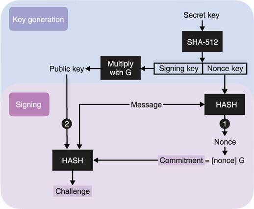
Figure 7.11 EdDSA key generation produces a secret key that is then used to derive two other keys. The first derived key is the actual signing key and can thus be used to derive the public key; the other derived key is the nonce key, used to deterministically derive the nonce during signing operations. EdDSA signatures are then like Schnorr signatures with the exception that (1) the nonce is generated deterministically from the nonce key and the message, and (2) the public key of the signer is included as part of the challenge.
Notice how the nonce (or ephemeral key) is derived deterministically and not probabilistically from the nonce key and the given message. This means that signing two different messages should involve two different nonces, ingeniously preventing the signer from reusing nonces and, in turn, leaking out the key (as can happen with ECDSA). Signing the same message twice produces the same nonce twice, which then produces the same signature twice as well. This is obviously not a problem. A signature can be verified by computing the following two equations:
R + [HASH(R || public key || message)] public key
The signature is valid if the two values match. This is exactly how Schnorr signatures work, except that we are now in an elliptic curve group and I use the additive notation here.
The most widely used instantiation of EdDSA, Ed25519, is defined with the Edwards25519 curve and the SHA-512 as a hash function. The Edwards25519 curve is defined with all the points satisfying this equation:
–x2 + y2 = 1 + d × x2 × y2 mod p
where the value d is the large number
37095705934669439343138083508754565189542113879843219016388785533085940283555
and the variables x and y are taken modulo p the large number 2255 – 19 (the same prime used for Curve25519). The base point is G of coordinate
x = 15112221349535400772501151409588531511454012693041857206046113283949847762202
y = 46316835694926478169428394003475163141307993866256225615783033603165251855960
RFC 8032 actually defines three variants of EdDSA using the Edwards25519 curve. All three variants follow the same key generation algorithm but with different signing and verification algorithms:
Ed25519 (or pureEd25519)—That’s the algorithm that I explained previously.
Ed25519ctx—This algorithm introduces a mandatory customization string and is rarely implemented, if even used, in practice. The only difference is that some user-chosen prefix is added to every call to the hash function.
Ed25519ph (or HashEd25519)—This allows applications to prehash the message before signing it (hence the ph in the name). It also builds on Ed25519ctx, allowing the caller to include an optional custom string.
The addition of a customization string is quite common in cryptography as you saw with some hash functions in chapter 2 or will see with key derivation functions in chapter 8. It is a useful addition when a participant in a protocol uses the same key to sign messages in different contexts. For example, you can imagine an application that would allow you to sign transactions using your private key and also to sign private messages to people you talk to. If you mistakenly sign and send a message that looks like a transaction to your evil friend Eve, she could try to republish it as a valid transaction if there’s no way to distinguish the two types of payload you’re signing.
Ed25519ph was introduced solely to please callers that need to sign large messages. As you saw in chapter 2, hash functions often provide an “init-update-finalize” interface that allows you to continuously hash a stream of data without having to keep the whole input in memory.
You are now done with your tour of the signature schemes used in real-world applications. Next, let’s look at how you can possibly shoot yourself in the foot when using these signature algorithms. But first, a recap:
RSA PKCS#1 v1.5 is still widely in use but is hard to implement correctly and many implementations have been found to be broken.
RSA-PSS has a proof of security, is easier to implement, but has seen poor adoption due to newer schemes based on elliptic curves.
ECDSA is the main competition to RSA PKCS#1 v1.5 and is mostly used with NIST’s curve P-256, except in the cryptocurrency world where Secp256k1 seems to dominate.
Ed25519 is based on Schnorr signatures, has received wide adoption, and it is easier to implement compared to ECDSA; it does not require new randomness for every signing operation. This is the algorithm you should use if you can.
There are a number of subtle properties that signature schemes might exhibit. While they might not matter in most protocols, not being aware of these “gotchas” can end up biting you when working on more complex and nonconventional protocols. The end of this chapter focuses on known issues with digital signatures.
A digital signature does not uniquely identify a key or a message.
—Andrew Ayer (“Duplicate Signature Key Selection Attack in Let’s Encrypt,” 2015)
Substitution attacks, also referred to as duplicate signature key selection (DSKS), are possible on both RSA PKCS#1 v1.5 and RSA-PSS. Two DSKS variants exist:
Key substitution attacks—A different key pair or public key is used to validate a given signature over a given message.
Message key substitution attacks—A different key pair or public key is used to validate a given signature over a new message.
One more time: the first attack fixes both the message and the signature; the second one only fixes the signature. I recapitulate this in figure 7.12.
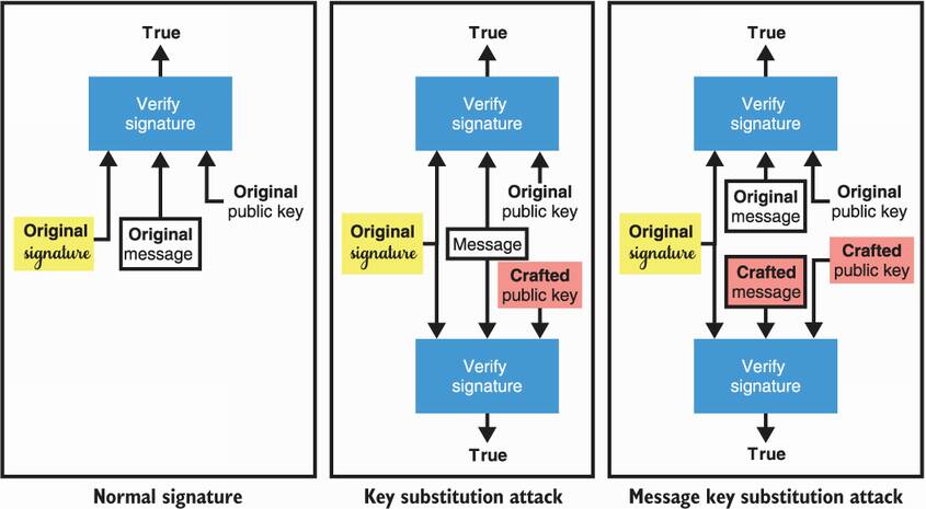
Figure 7.12 Signature algorithms like RSA are vulnerable to key substitution attacks, which are surprising and unexpected behaviors for most users of cryptography. A key substitution attack allows one to take a signature over a message and to craft a new key pair that validates the original signature. A variant called message key substitution allows an attacker to create a new key pair and a new message that validates under the original signature.
In February 2014 MtGox, once the largest Bitcoin exchange, closed and filed for bankruptcy claiming that attackers used malleability attacks to drain its accounts.
—Christian Decker and Roger Wattenhofer (“Bitcoin Transaction Malleability and MtGox,” 2014)
Most signature schemes are malleable: if you give me a valid signature, I can modify the signature so that it becomes a different, but still valid signature. I have no clue what the signing key was, yet I managed to create a new valid signature.
Non-malleability does not necessarily mean that signatures are unique: if I’m the signer, I can usually create different signatures for the same message and that’s usually OK. Some constructions like verifiable random functions (which you’ll see later in chapter 8) rely on signature uniqueness, and so they must deal with this or use signature schemes that have unique signatures (like the Boneh–Lynn–Shacham, or BLS, signatures).
What to do with all of this information? Rest assured, signature schemes are definitely not broken, and you probably shouldn’t worry if your use of signatures is not too out-of-the-box. But if you’re designing cryptographic protocols or if you’re implementing a protocol that’s more complicated than everyday cryptography, you might want to keep these subtle properties in the back of your mind.
Digital signatures are similar to pen-and-paper signatures but are backed with cryptography, making them unforgeable by anyone who does not control the signing (private) key.
Digital signatures can be useful to authenticate origins (for example, one side of a key exchange) as well as providing transitive trust (if I trust Alice and she trusts Bob, I can trust Bob).
Zero-knowledge proofs (ZKPs) allow a prover to prove the knowledge of a particular piece of information (called a witness), without revealing that something. Signatures can be seen as non-interactive ZKPs as they do not require the verifier to be online during the signing operation.
You can use many standards to sign:
Some subtle properties can be dangerous if signatures are used in a nonconventional way: