Chapter 9. Miscellaneous problems
Throughout this book we have covered a myriad of problem-solving techniques relevant to modern software development tasks. To study each technique, we have explored famous computer science problems. But not every famous problem fits the mold of the prior chapters. This chapter is a gathering point for famous problems that did not quite fit into any other chapter. Think of these problems as a bonus: more interesting problems with less scaffolding around them.
9.1. The knapsack problem
The knapsack problem is an optimization problem that takes a common computational need—finding the best use of limited resources given a finite set of usage options—and spins it into a fun story. A thief enters a home with the intent to steal. He has a knapsack, and he is limited in what he can steal by the capacity of the knapsack. How does he figure out what to put into the knapsack? The problem is illustrated in figure 9.1.
Figure 9.1. The burgler must decide what items to steal because the capacity of the knapsack is limited.
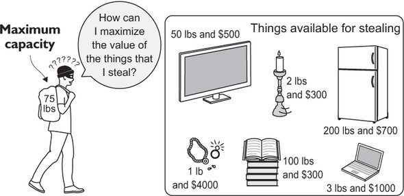
If the thief could take any amount of any item, he could simply divide each item’s value by its weight to figure out the most valuable items for the available capacity. But to make the scenario more realistic, let’s say that the thief cannot take half of an item (such as 2.5 televisions). Instead, we will come up with a way to solve the 0/1 variant of the problem, so-called because it enforces another rule: The thief may only take one or none of each item.
First, let’s define a NamedTuple to hold our items.
Listing 9.1. knapsack.py
from typing import NamedTuple, List

class Item(NamedTuple):
    name: str
    weight: int
    value: float
If we tried to solve this problem using a brute-force approach, we would look at every combination of items available to be put in the knapsack. For the mathematically inclined, this is known as a powerset, and a powerset of a set (in our case, the set of items) has 2^N different possible subsets, where N is the number of items. Therefore, we would need to analyze 2^N combinations (O(2^N)). This is okay for a small number of items, but it is untenable for a large number. Any approach that solves a problem using an exponential number of steps is an approach we want to avoid.
Instead, we will use a technique known as dynamic programming, which is similar in concept to memoization (chapter 1). Instead of solving a problem outright with a brute-force approach, in dynamic programming one solves subproblems that make up the larger problem, stores those results, and utilizes those stored results to solve the larger problem. As long as the capacity of the knapsack is considered in discrete steps, the problem can be solved with dynamic programming.
For instance, to solve the problem for a knapsack with a 3-pound capacity and three items, we can first solve the problem for a 1-pound capacity and one possible item, 2-pound capacity and one possible item, and 3-pound capacity and one possible item. We can then use the results of that solution to solve the problem for 1-pound capacity and two possible items, 2-pound capacity and two possible items, and 3-pound capacity and two possible items. Finally, we can solve for all three possible items.
All along the way we will fill in a table that tells us the best possible solution for each combination of items and capacity. Our function will first fill in the table and then figure out the solution based on the table.[1]
I studied several resources to write this solution, the most authoritative of which was Algorithms (Addison-Wesley, 1988), 2nd edition, by Robert Sedgewick (p. 596). I looked at several examples of the 0/1 knapsack problem on Rosetta Code, most notably the Python dynamic programming solution (http://mng.bz/kx8C), which this function is largely a port of, back from the Swift version of the book. (It went from Python to Swift and back to Python again.)
Listing 9.2. knapsack.py continued
def knapsack(items: List[Item], max_capacity: int) -> List[Item]:
    # build up dynamic programming table
    table: List[List[float]] = [[0.0 for _ in range(max_capacity + 1)] for _
     in range(len(items) + 1)]
    for i, item in enumerate(items):
        for capacity in range(1, max_capacity + 1):
            previous_items_value: float = table[i][capacity]
            if capacity >= item.weight: # item fits in knapsack
                value_freeing_weight_for_item: float = table[i][capacity -
     item.weight]
                # only take if more valuable than previous item
                table[i + 1][capacity] = max(value_freeing_weight_for_item +
     item.value, previous_items_value)
            else: # no room for this item
                table[i + 1][capacity] = previous_items_value
    # figure out solution from table
    solution: List[Item] = []
    capacity = max_capacity
    for i in range(len(items), 0, -1): # work backwards
        # was this item used?
        if table[i - 1][capacity] != table[i][capacity]:
            solution.append(items[i - 1])
            # if the item was used, remove its weight
            capacity -= items[i - 1].weight
    return solution
The inner loop of the first part of this function will execute N * C times, where N is the number of items and C is the maximum capacity of the knapsack. Therefore, the algorithm performs in O(N * C) time, a significant improvement over the brute-force approach for a large number of items. For instance, for the 11 items that follow, a brute-force algorithm would need to examine 2^11 or 2,048 combinations. The preceding dynamic programming function will execute 825 times, because the maximum capacity of the knapsack in question is 75 arbitrary units (11 * 75). This difference would grow exponentially with more items.
Let’s look at the solution in action.
Listing 9.3. knapsack.py continued
if __name__ == "__main__":
    items: List[Item] = [Item("television", 50, 500),
                         Item("candlesticks", 2, 300),
                         Item("stereo", 35, 400),
                         Item("laptop", 3, 1000),
                         Item("food", 15, 50),
                         Item("clothing", 20, 800),
                         Item("jewelry", 1, 4000),
                         Item("books", 100, 300),
                         Item("printer", 18, 30),
                         Item("refrigerator", 200, 700),
                         Item("painting", 10, 1000)]
    print(knapsack(items, 75))
If you inspect the results printed to the console, you will see that the optimal items to take are the painting, jewelry, clothing, laptop, stereo, and candlesticks. Here’s some sample output showing the most valuable items for the thief to steal, given the limited-capacity knapsack:
[Item(name='painting', weight=10, value=1000), Item(name='jewelry', weight=1,
     value=4000), Item(name='clothing', weight=20, value=800),
     Item(name='laptop', weight=3, value=1000), Item(name='stereo',
     weight=35, value=400), Item(name='candlesticks', weight=2, value=300)]
To get a better idea of how this all works, let’s look at some of the particulars of the function:
for i, item in enumerate(items):
    for capacity in range(1, max_capacity + 1):
For each possible number of items, we loop through all of the capacities in a linear fashion, up to the maximum capacity of the knapsack. Notice that I say “each possible number of items” instead of each item. When i equals 2, it does not just represent item 2. It represents the possible combinations of the first two items for every explored capacity. item is the next item that we are considering stealing:
previous_items_value: float = table[i][capacity]
if capacity >= item.weight: # item fits in knapsack
previous_items_value is the value of the last combination of items at the current capacity being explored. For each possible combination of items, we consider whether adding in the latest “new” item is even possible.
If the item weighs more than the knapsack capacity we are considering, we simply copy over the value for the last combination of items that we considered for the capacity in question:
else: # no room for this item
    table[i + 1][capacity] = previous_items_value
Otherwise, we consider whether adding in the “new” item will result in a higher value than the last combination of items at that capacity that we considered. We do this by adding the value of the item to the value already computed in the table for the previous combination of items at a capacity equal to the item’s weight, subtracted from the current capacity we are considering. If this value is higher than the last combination of items at the current capacity, we insert it; otherwise, we insert the last value:
value_freeing_weight_for_item: float = table[i][capacity - item.weight]
# only take if more valuable than previous item
table[i + 1][capacity] = max(value_freeing_weight_for_item + item.value,
     previous_items_value)
That concludes building up the table. To actually find which items are in the solution, though, we need to work backward from the highest capacity and the final explored combination of items:
for i in range(len(items), 0, -1): # work backwards
    # was this item used?
    if table[i - 1][capacity] != table[i][capacity]:
We start from the end and loop through our table from right to left, checking whether there was a change in the value inserted into the table at each stop. If there was, that means we added the new item that was considered in a particular combination because the combination was more valuable than the prior one. Therefore, we add that item to the solution. Also, capacity is decreased by the weight of the item, which can be thought of as moving up the table:
solution.append(items[i - 1])
# if the item was used, remove its weight
capacity -= items[i - 1].weight
Note
Throughout both the build-up of the table and the solution search, you may have noticed some manipulation of iterators and table size by 1. This is done for convenience from a programmatic perspective. Think about how the problem is built from the bottom up. When the problem begins, we are dealing with a zero-capacity knapsack. If you work your way up from the bottom in a table, it will become clear why we need the extra row and column.
Are you still confused? Table 9.1 is the table the knapsack() function builds. It would be quite a large table for the preceding problem, so instead, let’s look at a table for a knapsack with 3-pound capacity and three items: matches (1 pound), flashlight (2 pounds), and book (1 pound). Assume those items are valued at $5, $10, and $15, respectively.
Table 9.1. An example of a knapsack problem of three items
|
0 lb. |
1 lb. |
2 lb. |
3 lb. |
|
|---|---|---|---|---|
| Matches (1 lb., $5) | 0 | 5 | 5 | 5 |
| Flashlight (2 lbs., $10) | 0 | 5 | 10 | 15 |
| Book (1 lb., $15) | 0 | 15 | 20 | 25 |
As you look across the table from left to right, the weight is increasing (how much you are trying to fit in the knapsack). As you look down the table from top to bottom, the number of items you are attempting to fit is increasing. On the first row, you are only trying to fit the matches. On the second row, you fit the most valuable combination of the matches and the flashlight that the knapsack can hold. On the third row, you fit the most valuable combination of all three items.
As an exercise to facilitate your understanding, try filling in a blank version of this table yourself, using the algorithm described in the knapsack() function with these same three items. Then use the algorithm at the end of the function to read back the right items from the table. This table corresponds to the table variable in the function.
9.2. The Traveling Salesman Problem
The Traveling Salesman Problem is one of the most classic and talked-about problems in all of computing. A salesman must visit all of the cities on a map exactly once, returning to his start city at the end of the journey. There is a direct connection from every city to every other city, and the salesman may visit the cities in any order. What is the shortest path for the salesman?
The problem can be thought of as a graph problem (chapter 4), with the cities being the vertices and the connections between them being the edges. Your first instinct might be to find the minimum spanning tree, as described in chapter 4. Unfortunately, the solution to the Traveling Salesman Problem is not so simple. The minimum spanning tree is the shortest way to connect all of the cities, but it does not provide the shortest path for visiting all of them exactly once.
Although the problem, as posed, appears fairly simple, there is no algorithm that can solve it quickly for an arbitrary number of cities. What do I mean by “quickly”? I mean that the problem is what is known as NP hard. An NP-hard (non-deterministic polynomial hard) problem is a problem for which no polynomial time algorithm exists. (The time it takes is a polynomial function of the size of the input.) As the number of cities that the salesman needs to visit increases, the difficulty of solving the problem grows exceptionally quickly. It is much harder to solve the problem for 20 cities than 10. It is impossible (to the best of current knowledge), in a reasonable amount of time, to solve the problem perfectly (optimally) for millions of cities.
Note
The naive approach to the Traveling Salesman Problem is O(n!). Why this is the case is discussed in section 9.2.2. We suggest reading section 9.2.1 before reading 9.2.2, though, because the implementation of a naive solution to the problem will make its complexity obvious.
9.2.1. The naive approach
The naive approach to the problem is simply to try every possible combination of cities. Attempting the naive approach will illustrate the difficulty of the problem and this approach’s unsuitability for brute-force attempts at larger scales.
Our sample data
In our version of the Traveling Salesman Problem, the salesman is interested in visiting five of the major cities of Vermont. We will not specify a starting (and therefore ending) city. Figure 9.2 illustrates the five cities and the driving distances between them. Note that there is a distance listed for the route between every pair of cities.
Figure 9.2. Five cities in Vermont and the driving distances between them
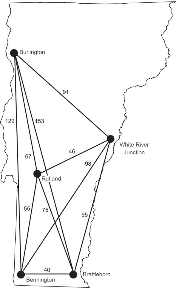
Perhaps you have seen driving distances in table form before. In a driving-distance table, one can easily look up the distance between any two cities. Table 9.2 lists the driving distances for the five cities in the problem.
Table 9.2. Driving distances between cities in Vermont
|
Rutland |
Burlington |
White River Junction |
Bennington |
Brattleboro |
|
|---|---|---|---|---|---|
| Rutland | 0 | 67 | 46 | 55 | 75 |
| Burlington | 67 | 0 | 91 | 122 | 153 |
| White River Junction | 46 | 91 | 0 | 98 | 65 |
| Bennington | 55 | 122 | 98 | 0 | 40 |
| Brattleboro | 75 | 153 | 65 | 40 | 0 |
We will need to codify both the cities and the distances between them for our problem. To make the distances between cities easy to look up, we will use a dictionary of dictionaries, with the outer set of keys representing the first of a pair and the inner set of keys representing the second. This will be the type Dict[str, Dict[str, int]], and it will allow lookups like vt_distances["Rutland"]["Burlington"], which should return 67.
Listing 9.4. tsp.py
from typing import Dict, List, Iterable, Tuple
from itertools import permutations

vt_distances: Dict[str, Dict[str, int]] = {
    "Rutland":
        {"Burlington": 67,
         "White River Junction": 46,
         "Bennington": 55,
         "Brattleboro": 75},
    "Burlington":
        {"Rutland": 67,
         "White River Junction": 91,
         "Bennington": 122,
         "Brattleboro": 153},
    "White River Junction":
        {"Rutland": 46,
         "Burlington": 91,
         "Bennington": 98,
         "Brattleboro": 65},
    "Bennington":
        {"Rutland": 55,
         "Burlington": 122,
         "White River Junction": 98,
         "Brattleboro": 40},
    "Brattleboro":
        {"Rutland": 75,
         "Burlington": 153,
         "White River Junction": 65,
         "Bennington": 40}
}
Finding all permutations
The naive approach to solving the Traveling Salesman Problem requires generating every possible permutation of the cities. There are many permutation-generation algorithms; they are simple enough to ideate that you could almost certainly come up with one on your own.
One common approach is backtracking. You first saw backtracking in chapter 3 in the context of solving a constraint-satisfaction problem. In constraint-satisfaction problem solving, backtracking is used after a partial solution is found that does not satisfy the problem’s constraints. In such a case, you revert to an earlier state and continue the search along a different path than that which led to the incorrect partial solution.
To find all of the permutations of the items in a list (say, our cities), you could also use backtracking. After making a swap between elements to go down a path of further permutations, you can backtrack to the state before the swap was made so that a different swap can be made in order to go down a different path.
Luckily, there is no need to reinvent the wheel by writing a permutation-generation algorithm, because the Python standard library has a permutations() function in its itertools module. In the following code snippet, we generate all of the permutations of the Vermont cities that our travelling salesman would need to visit. Because there are five cities, this is 5! (5 factorial), or 120 permutations.
Listing 9.5. tsp.py continued
vt_cities: Iterable[str] = vt_distances.keys()
city_permutations: Iterable[Tuple[str, ...]] = permutations(vt_cities)
Brute-force search
We can now generate all of the permutations of the city list, but this is not quite the same as a Traveling Salesman Problem path. Recall that in the Traveling Salesman Problem, the salesman must return, at the end, to the same city that he started in. We can easily add the first city in a permutation to the end of a permutation using a list comprehension.
Listing 9.6. tsp.py continued
tsp_paths: List[Tuple[str, ...]] = [c + (c[0],) for c in city_permutations]
We are now ready to try testing the paths we have permuted. A brute-force search approach painstakingly looks at every path in a list of paths and uses the distance between two cities lookup table (vt_distances) to calculate each path’s total distance. It prints both the shortest path and that path’s total distance.
Listing 9.7. tsp.py continued
if __name__ == "__main__":
    best_path: Tuple[str, ...]
    min_distance: int = 99999999999 # arbitrarily high number
    for path in tsp_paths:
        distance: int = 0
        last: str = path[0]
        for next in path[1:]:
            distance += vt_distances[last][next]
            last = next
        if distance < min_distance:
            min_distance = distance
            best_path = path
    print(f"The shortest path is {best_path} in {min_distance} miles.")
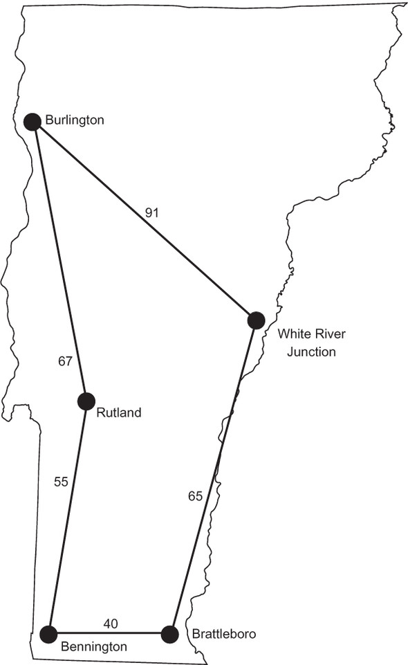
We finally can brute-force the cities of Vermont, finding the shortest path to reach all five. The output should look something like the following, and the best path is illustrated in figure 9.3.
The shortest path is ('Rutland', 'Burlington', 'White River Junction',
     'Brattleboro', 'Bennington', 'Rutland') in 318 miles.
Figure 9.3. The shortest path for the salesman to visit all five cities in Vermont is illustrated.
9.2.2. Taking it to the next level
There is no easy answer to the Traveling Salesman Problem. Our naive approach quickly becomes infeasible. The number of permutations generated is n factorial (n!), where n is the number of cities in the problem. If we were to include just one more city (six instead of five), the number of evaluated paths would grow by a factor of six. Then it would be seven times harder to solve the problem for just one more city after that. This is not a scalable approach!
In the real world, the naive approach to the Traveling Salesman Problem is seldom used. Most algorithms for instances of the problem with a large number of cities are approximations. They try to solve the problem for a near-optimal solution. The near-optimal solution may be within a small known band of the perfect solution. (For example, perhaps they will be no more than 5% less efficient.)
Two techniques that have already appeared in this book have been used to attempt the Traveling Salesman Problem on large data sets. Dynamic programming, which we used in the knapsack problem earlier in this chapter, is one approach. Another is genetic algorithms, as described in chapter 5. Many journal articles have been published attributing genetic algorithms to near-optimal solutions for the traveling salesman with large numbers of cities.
9.3. Phone number mnemonics
Before there were smartphones with built-in address books, telephones included letters on each of the keys on their number pads. The reason for these letters was to provide easy mnemonics by which to remember phone numbers. In the United States, typically the 1 key would have no letters, 2 would have ABC, 3 DEF, 4 GHI, 5 JKL, 6 MNO, 7 PQRS, 8 TUV, 9 WXYZ, and 0 no letters. For example, 1-800-MY-APPLE corresponds to the phone number 1-800-69-27753. Once in a while you will still find these mnemonics in advertisements, so the numbers on the keypad have made their way into modern smartphone apps, as evidenced by figure 9.4.
Figure 9.4. The Phone app in iOS retains the letters on keys that its telephone forebears contained.

How does one come up with a new mnemonic for a phone number? In the 1990s there was popular shareware to help with the effort. These pieces of software would generate every permutation of a phone number’s letters and then look through a dictionary to find words that were contained in the permutations. They would then show the permutations with the most complete words to the user. We will do the first half of the problem. The dictionary lookup will be left as an exercise.
In the last problem, when we looked at permutation generation, we used the permutations() function to generate the potential paths for the Traveling Salesman Problem. However, as was mentioned, there are many different ways to generate permutations. For this problem in particular, instead of swapping two positions in an existing permutation to generate a new one, we will generate each permutation from the ground up. We will do this by looking at the potential letters that match each numeral in the phone number and continually add more options to the end as we go to each successive numeral. This is a kind of Cartesian product, and once again, the Python standard library’s itertools module has us covered.
First, we will define a mapping of numerals to potential letters.
Listing 9.8. tsp.py continued
from typing import Dict, Tuple, Iterable, List
from itertools import product

phone_mapping: Dict[str, Tuple[str, ...]] = {"1": ("1",),
                                             "2": ("a", "b", "c"),
                                             "3": ("d", "e", "f"),
                                             "4": ("g", "h", "i"),
                                             "5": ("j", "k", "l"),
                                             "6": ("m", "n", "o"),
                                             "7": ("p", "q", "r", "s"),
                                             "8": ("t", "u", "v"),
                                             "9": ("w", "x", "y", "z"),
                                             "0": ("0",)}
The next function combines all of those possibilities for each numeral into a list of possible mnemonics for a given phone number. It does this by creating a list of tuples of potential letters for each digit in the phone number and then combining them through the Cartesian product function product() from itertools. Note the use of the unpack (*) operator to use the tuples in letter_tuples as the arguments for product().
Listing 9.9. tsp.py continued
def possible_mnemonics(phone_number: str) -> Iterable[Tuple[str, ...]]:
    letter_tuples: List[Tuple[str, ...]] = []
    for digit in phone_number:
        letter_tuples.append(phone_mapping.get(digit, (digit,)))
    return product(*letter_tuples)
Now we can find all of the possible mnemonics for a phone number.
Listing 9.10. tsp.py continued
if __name__ == "__main__":
    phone_number: str = input("Enter a phone number:")
    print("Here are the potential mnemonics:")
for mnemonic in possible_mnemonics(phone_number):
    print("".join(mnemonic))
It turns out that the phone number 1440787 can also be written as 1GH0STS. That is easier to remember.
9.4. Real-world applications
Dynamic programming, as used with the knapsack problem, is a widely applicable technique that can make seemingly intractable problems solvable by breaking them into constituent smaller problems and building up a solution from those parts. The knapsack problem itself is related to other optimization problems where a finite amount of resources (the capacity of the knapsack) must be allocated amongst a finite but exhaustive set of options (the items to steal). Imagine a college that needs to allocate its athletic budget. It does not have enough money to fund every team, and it has some expectation of how much alumni donations each team will bring in. It can run a knapsack-like problem to optimize the budget’s allocation. Problems like this are common in the real world.
The Traveling Salesman Problem is an everyday occurrence for shipping and distribution companies like UPS and FedEx. Package delivery companies want their drivers to travel the shortest routes possible. Not only does this make the drivers’ jobs more pleasant, but it also saves fuel and maintenance costs. We all travel for work or for pleasure, and finding optimal routes when visiting many destinations can save resources. But the Traveling Salesman Problem is not just for routing travel; it comes up in almost any routing scenario that requires singular visits to nodes. Although a minimum spanning tree (chapter 4) may minimize the amount of wire needed to connect a neighborhood, it does not tell us the optimal amount of wire if every house must be forward-connected to just one other house as part of a giant circuit that returns to its origination. The Traveling Salesman Problem does.
Permutation-generation techniques like the ones used in the naive approach to the Traveling Salesman Problem and the phone number mnemonics problem are useful for testing all sorts of brute-force algorithms. For instance, if you were trying to crack a short password, you could generate every possible permutation of the characters that could potentially be in the password. Practitioners of such large-scale permutation-generation tasks would be wise to use an especially efficient permutation-generation algorithm like Heap’s algorithm.[2]
Robert Sedgewick, “Permutation Generation Methods” (Princeton University), http://mng.bz/87Te.
9.5. Exercises
- Reprogram the naive approach to the Traveling Salesman Problem, using the graph framework from chapter 4.
- Implement a genetic algorithm, as described in chapter 5, to solve the Traveling Salesman Problem. Start with the simple data set of Vermont cities described in this chapter. Can you get the genetic algorithm to arrive at the optimal solution in a short amount of time? Then attempt the problem with an increasingly large number of cities. How well does the genetic algorithm hold up? You can find a large number of data sets specifically made for the Traveling Salesman Problem by searching the web. Develop a testing framework for checking the efficiency of your method.
- Use a dictionary with the phone number mnemonics program and return only permutations that contain valid dictionary words.