Chapter 7. Fairly simple neural networks
When we hear about advances in artificial intelligence these days, in the late 2010s, they generally concern a particular subdiscipline known as machine learning (computers learning some new information without being explicitly told it). More often than not those advances are being driven by a particular machine-learning technique known as neural networks. Although invented decades ago, neural networks have been going through a kind of renaissance as improved hardware and newly discovered research-driven software techniques enable a new paradigm known as deep learning.
Deep learning has turned out to be a broadly applicable technique. It has been found useful in everything from hedge-fund algorithms to bioinformatics. Two deep-learning applications that consumers have become familiar with are image recognition and speech recognition. If you have ever asked your digital assistant what the weather is or had a photo program recognize your face, there was probably some deep learning going on.
Deep-learning techniques utilize the same building blocks as simpler neural networks. In this chapter we will explore those blocks by building a simple neural network. It will not be state of the art, but it will give you a basis for understanding deep learning (which is based on more complex neural networks than we will build). Most practitioners of machine learning do not build neural networks from scratch. Instead, they use popular, highly optimized, off-the-shelf frameworks that do the heavy lifting. Although this chapter will not help you learn how to use any specific framework, and the network we will build will not be useful for an actual application, it will help you understand how those frameworks work at a low level.
7.1. Biological basis?
The human brain is the most incredible computational device in existence. It cannot crunch numbers as fast as a microprocessor, but its ability to adapt to new situations, learn new skills, and be creative is unsurpassed by any known machine. Since the dawn of computers, scientists have been interested in modeling the brain’s machinery. Each nerve cell in the brain is known as a neuron. Neurons in the brain are networked to one another via connections known as synapses. Electricity passes through synapses to power these networks of neurons—also known as neural networks.
Note
The preceding description of biological neurons is a gross oversimplification for analogy’s sake. In fact, biological neurons have parts like axons, dendrites, and nuclei that you may remember from high-school biology. And synapses are actually gaps between neurons where neurotransmitters are secreted to enable those electrical signals to pass.
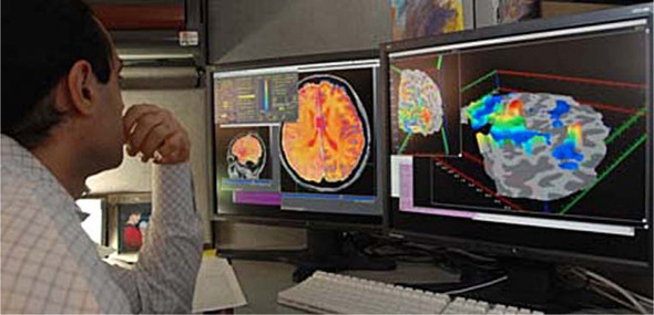
Although scientists have identified the parts and functions of neurons, the details of how biological neural networks form complex thought patterns are still not well understood. How do they process information? How do they form original thoughts? Most of our knowledge of how the brain works comes from looking at it on a macro level. Functional magnetic resonance imaging (fMRI) scans of the brain show where blood flows when a human is doing a particular activity or thinking a particular thought (illustrated in figure 7.1). This and other macro-techniques can lead to inferences about how the various parts are connected, but they do not explain the mysteries of how individual neurons aid in the development of new thoughts.
Figure 7.1. A researcher studies fMRI images of the brain. fMRI images do not tell us much about how individual neurons function or how neural networks are organized.
Teams of scientists are racing around the globe to unlock the brain’s secrets, but consider this: The human brain has approximately 100,000,000,000 neurons, and each of them may have connections with as many as tens of thousands of other neurons. Even for a computer with billions of logic gates and terabytes of memory, a single human brain would be impossible to model using today’s technology. Humans will still likely be the most advanced general-purpose learning entities for the foreseeable future.
Note
A general-purpose learning machine that is equivalent to human beings in abilities is the goal of so-called strong AI (also known as artificial general intelligence). At this point in history, it is still the stuff of science fiction. Weak AI is the type of AI you see every day: computers intelligently solving specific tasks they were preconfigured to accomplish.
If biological neural networks are not fully understood, then how has modeling them been an effective computational technique? Although digital neural networks, known as artificial neural networks, are inspired by biological neural networks, inspiration is where the similarities end. Modern artificial neural networks do not claim to work like their biological counterparts. In fact, that would be impossible, because we do not completely understand how biological neural networks work to begin with.
7.2. Artificial neural networks
In this section we will look at what is arguably the most common type of artificial neural network, a feed-forward network with backpropagation—the same type we will later be developing. Feed-forward means the signal is generally moving in one direction through the network. Backpropagation means we will determine errors at the end of each signal’s traversal through the network and try to distribute fixes for those errors back through the network, especially affecting the neurons that were most responsible for them. There are many other types of artificial neural networks, and perhaps this chapter will pique your interest in exploring further.
7.2.1. Neurons
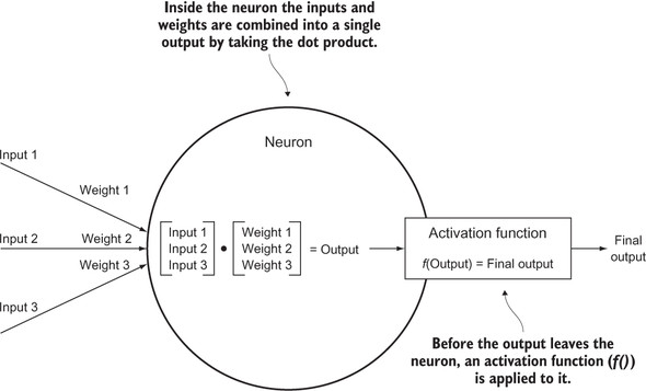
The smallest unit in an artificial neural network is a neuron. It holds a vector of weights, which are just floating-point numbers. A vector of inputs (also just floating-point numbers) is passed to the neuron. It combines those inputs with its weights using a dot product. It then runs an activation function on that product and spits the result out as its output. This action can be thought of as analagous to a real neuron firing.
An activation function is a transformer of the neuron’s output. The activation function is almost always nonlinear, which allows neural networks to represent solutions to nonlinear problems. If there were no activation functions, the entire neural network would just be a linear transformation. Figure 7.2 shows a single neuron and its operation.
Figure 7.2. A single neuron combines its weights with input signals to produce an output signal that is modified by an activation function.
Note
There are some math terms in this section that you may not have seen since a precalculus or linear algebra class. Explaining what vectors or dot products are is beyond the scope of this chapter, but you will likely get an intuition of what a neural network does by following along in this chapter, even if you do not understand all of the math. Later in the chapter there will be some calculus, including the use of derivatives and partial derivatives, but even if you do not understand all of the math, you should be able to follow the code. In fact, this chapter will not explain how to derive the formulas using calculus. Instead, it will focus on using the derivations.
7.2.2. Layers
In a typical feed-forward artificial neural network, neurons are organized in layers. Each layer consists of a certain number of neurons lined up in a row or column (depending on the diagram; the two are equivalent). In a feed-forward network, which is what we will be building, signals always pass in a single direction from one layer to the next. The neurons in each layer send their output signal to be used as input to the neurons in the next layer. Every neuron in each layer is connected to every neuron in the next layer.
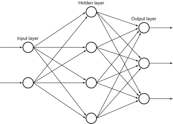
The first layer is known as the input layer, and it receives its signals from some external entity. The last layer is known as the output layer, and its output typically must be interpreted by an external actor to get an intelligent result. The layers between the input and output layers are known as hidden layers. In simple neural networks like the one we will be building in this chapter, there is just one hidden layer, but deep-learning networks have many. Figure 7.3 shows the layers working together in a simple network. Note how the outputs from one layer are used as the inputs to every neuron in the next layer.
Figure 7.3. A simple neural network with one input layer of two neurons, one hidden layer of four neurons, and one output layer of three neurons. The number of neurons in each layer in this figure is arbitrary.
These layers just manipulate floating-point numbers. The inputs to the input layer are floating-point numbers, and the outputs from the output layer are floating-point numbers.
Obviously, these numbers must represent something meaningful. Imagine that the network was designed to classify small black-and-white images of animals. Perhaps the input layer has 100 neurons representing the grayscale intensity of each pixel in a 10 x 10 pixel animal image, and the output layer has 5 neurons representing the likelihood that the image is of a mammal, reptile, amphibian, fish, or bird. The final classification could be determined by the output neuron with the highest floating-point output. If the output numbers were 0.24, 0.65, 0.70, 0.12, and 0.21, respectively, the image would be determined to be an amphibian.
7.2.3. Backpropagation
The last piece of the puzzle, and the inherently most complex part, is backpropagation. Backpropagation finds the error in a neural network’s output and uses it to modify the weights of neurons. The neurons most responsible for the error are most heavily modified. But where does the error come from? How can we know the error? The error comes from a phase in the use of a neural network known as training.
Tip
There are steps written out (in English) for several mathematical formulas in this section. Pseudo formulas (not using proper notation) are in the accompanying figures. This approach will make the formulas readable for those uninitiated in (or out of practice with) mathematical notation. If the more formal notation (and the derivation of the formulas) interests you, check out chapter 18 of Norvig and Russell’s Artificial Intelligence.[1]
Stuart Russell and Peter Norvig, Artificial Intelligence: A Modern Approach, 3rd edition (Pearson, 2010).
Before they can be used, most neural networks must be trained. We must know the right outputs for some inputs so that we can use the difference between expected outputs and actual outputs to find errors and modify weights. In other words, neural networks know nothing until they are told the right answers for a certain set of inputs, so that they can prepare themselves for other inputs. Backpropagation only occurs during training.
Note
Because most neural networks must be trained, they are considered a type of supervised machine learning. Recall from chapter 6 that the k-means algorithm and other cluster algorithms are considered a form of unsupervised machine learning because once they are started, no outside intervention is required. There are other types of neural networks than the one described in this chapter that do not require pretraining and are considered a form of unsupervised learning.
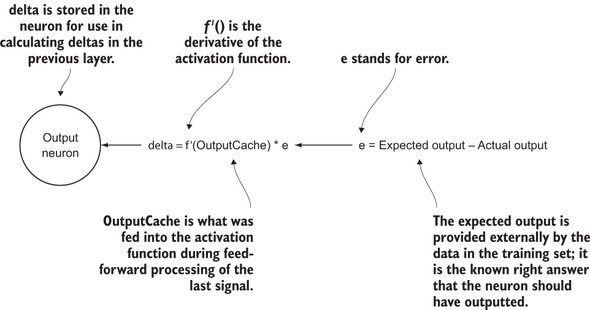
The first step in backpropagation is to calculate the error between the neural network’s output for some input and the expected output. This error is spread across all of the neurons in the output layer. (Each neuron has an expected output and its actual output.) The derivative of the output neuron’s activation function is then applied to what was output by the neuron before its activation function was applied. (We cache its pre-activation function output.) This result is multiplied by the neuron’s error to find its delta. This formula for finding the delta uses a partial derivative, and its calculus derivation is beyond the scope of this book, but we are basically figuring out how much of the error each output neuron was responsible for. See figure 7.4 for a diagram of this calculation.
Figure 7.4. The mechanism by which an output neuron’s delta is calculated during the backpropagation phase of training
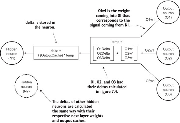
Deltas must then be calculated for every neuron in the hidden layer(s) in the network. We must determine how much each neuron was responsible for the incorrect output in the output layer. The deltas in the output layer are used to calculate the deltas in the preceding hidden layer. For each previous layer, the deltas are calculated by taking the dot product of the next layer’s weights with respect to the particular neuron in question and the deltas already calculated in the next layer. This value is multiplied by the derivative of the activation function applied to a neuron’s last output (cached before the activation function was applied) to get the neuron’s delta. Again, this formula is derived using a partial derivative, which you can read about in more mathematically focused texts.
Figure 7.5 shows the actual calculation of deltas for neurons in hidden layers. In a network with multiple hidden layers, neurons O1, O2, and O3 could be neurons in the next hidden layer instead of in the output layer.
Figure 7.5. How a delta is calculated for a neuron in a hidden layer
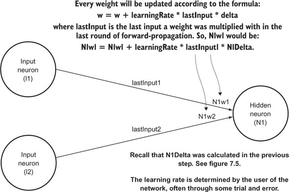
Last, but most important, all of the weights for every neuron in the network must be updated by multiplying each individual weight’s last input with the delta of the neuron and something called a learning rate, and adding that to the existing weight. This method of modifying the weight of a neuron is known as gradient descent. It is like climbing down a hill representing the error function of the neuron toward a point of minimal error. The delta represents the direction we want to climb, and the learning rate affects how fast we climb. It is hard to determine a good learning rate for an unknown problem without trial and error. Figure 7.6 shows how every weight in the hidden layer and output layer is updated.
Figure 7.6. The weights of every hidden layer and output layer neuron are updated using the deltas calculated in the previous steps, the prior weights, the prior inputs, and a user-determined learning rate.
Once the weights are updated, the neural network is ready to be trained again with another input and expected output. This process repeats until the network is deemed well trained by the neural network’s user. This can be determined by testing it against inputs with known correct outputs.
Backpropagation is complicated. Do not worry if you do not yet grasp all of the details. The explanation in this section may not be enough. Ideally, implementing backpropagation will take your understanding to the next level. As we implement our neural network and backpropagation, keep in mind this overarching theme: Backpropagation is a way of adjusting each individual weight in the network according to its responsibility for an incorrect output.
7.2.4. The big picture
We covered a lot of ground in this section. Even if the details do not yet make sense, it is important to keep the main themes in mind for a feed-forward network with backpropagation:
- Signals (floating-point numbers) move through neurons organized in layers in one direction. Every neuron in each layer is connected to every neuron in the next layer.
- Each neuron (except in the input layer) processes the signals it receives by combining them with weights (also floating-point numbers) and applying an activation function.
- During a process called training, network outputs are compared with expected outputs to calculate errors.
- Errors are backpropagated through the network (back toward where they came from) to modify weights so that they are more likely to create correct outputs.
There are more methods for training neural networks than the one explained here. There are also many other ways for signals to move within neural networks. The method explained here, and that we will be implementing, is just a particularly common form that serves as a decent introduction. Appendix B lists further resources for learning more about neural networks (including other types) and the math.
7.3. Preliminaries
Neural networks utilize mathematical mechanisms that require a lot of floating-point operations. Before we develop the actual structures of our simple neural network, we will need some mathematical primitives. These simple primitives are used extensively in the code that follows, so if you can find ways to accelerate them, it will really improve the performance of your neural network.
Warning
The complexity of the code in this chapter is arguably greater than any other in the book. There is a lot of build-up, with actual results seen only at the very end. There are many resources about neural networks that help you build one in very few lines of code, but this example is aimed at exploring the machinery and how the different components work together in a readable and extensible fashion. That is our goal, even if the code is a little longer and more expressive.
7.3.1. Dot product
As you will recall, dot products are required both for the feed-forward phase and for the backpropagation phase. Luckily, a dot product is simple to implement using the Python built-in functions zip() and sum(). We will keep our preliminary functions in a util.py file.
Listing 7.1. util.py
from typing import List
from math import exp

# dot product of two vectors
def dot_product(xs: List[float], ys: List[float]) -> float:
    return sum(x * y for x, y in zip(xs, ys))
7.3.2. The activation function
Recall that the activation function transforms the output of a neuron before the signal passes to the next layer (see figure 7.2). The activation function has two purposes: It allows the neural network to represent solutions that are not just linear transformations (as long as the activation function itself is not just a linear transformation), and it can keep the output of each neuron within a certain range. An activation function should have a computable derivative so that it can be used for backpropagation.
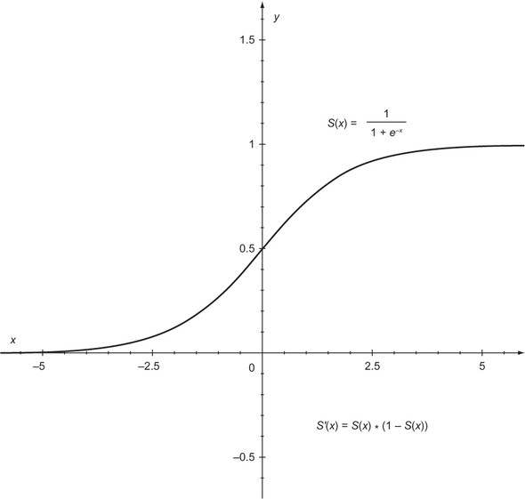
Sigmoid functions are a popular set of activation functions. One particularly popular sigmoid function (often just referred to as “the sigmoid function”) is illustrated in figure 7.7 (referred to in the figure as S(x)), along with its equation and derivative (S'(x)). The result of the sigmoid function will always be a value between 0 and 1. Having the value consistently be between 0 and 1 is useful for the network, as you will see. You will shortly see the formulas from the figure written out in code.
There are other activation functions, but we will use the sigmoid function. Here is a straightforward conversion of the formulas in figure 7.7 into code:
Figure 7.7. The sigmoid activation function (S(x)) will always return a value between 0 and 1. Note that its derivative is easy to compute as well (S'(x)).
Listing 7.2. util.py continued
# the classic sigmoid activation function
def sigmoid(x: float) -> float:
    return 1.0 / (1.0 + exp(-x))

def derivative_sigmoid(x: float) -> float:
    sig: float = sigmoid(x)
    return sig * (1 - sig)
7.4. Building the network
We will create classes to model all three organizational units in the network: neurons, layers, and the network itself. For the sake of simplicity, we will start from the smallest (neurons), move to the central organizing component (layers), and build up to the largest (the whole network). As we go from smallest component to largest component, we will encapsulate the previous level. Neurons only know about themselves. Layers know about the neurons they contain and other layers. And the network knows about all of the layers.
Note
There are many long lines of code in this chapter that do not neatly fit in the column limits of a printed book. I strongly recommend downloading the source code for this chapter from the book’s source code repository and following along on your computer screen as you read: https://github.com/davecom/ClassicComputerScienceProblemsInPython.
7.4.1. Implementing neurons
Let’s start with a neuron. An individual neuron will store many pieces of state, including its weights, its delta, its learning rate, a cache of its last output, and its activation function, along with the derivative of that activation function. Some of these elements could be more efficiently stored up a level (in the future Layer class), but they are included in the following Neuron class for illustrative purposes.
Listing 7.3. neuron.py
from typing import List, Callable
from util import dot_product

class Neuron:
def __init__(self, weights: List[float], learning_rate: float,
 activation_function: Callable[[float], float], derivative_activation_
 function: Callable[[float], float]) -> None:
    self.weights: List[float] = weights
    self.activation_function: Callable[[float], float] = activation_
 function
    self.derivative_activation_function: Callable[[float], float] =
 derivative_activation_function
    self.learning_rate: float = learning_rate
    self.output_cache: float = 0.0
    self.delta: float = 0.0

def output(self, inputs: List[float]) -> float:
    self.output_cache = dot_product(inputs, self.weights)
    return self.activation_function(self.output_cache)
Most of these parameters are initialized in the __init__() method. Because delta and output_cache are not known when a Neuron is first created, they are just initialized to 0. All of the neuron’s variables are mutable. In the life of the neuron (as we will be using it) their values may never change, but there is still a reason to make them mutable: flexibility. If this Neuron class were to be used with other types of neural networks, it is possible that some of these values might change on the fly. There are neural networks that change the learning rate as the solution approaches and that automatically try different activation functions. Here, we are trying to keep the Neuron class maximally flexible for other neural network applications.
The only other method, other than __init__(), is output(). output() takes the input signals (inputs) coming to the neuron and applies the formula discussed earlier in the chapter (see figure 7.2). The input signals are combined with the weights via a dot product, and this is cached in output_cache. Recall from the section on backpropagation that this value, obtained before the activation function is applied, is used to calculate delta. Finally, before the signal is sent on to the next layer (by being returned from output()), the activation function is applied to it.
That is it! An individual neuron in this network is fairly simple. It cannot do much beyond take an input signal, transform it, and send it off to be processed further. It maintains several elements of state that are used by the other classes.
7.4.2. Implementing layers
A layer in our network will need to maintain three pieces of state: its neurons, the layer that preceded it, and an output cache. The output cache is similar to that of a neuron, but up one level. It caches the outputs (after activation functions are applied) of every neuron in the layer.
At creation time, a layer’s main responsibility is to initialize its neurons. Our Layer class’s __init__() method therefore needs to know how many neurons it should be initializing, what their activation functions should be, and what their learning rates should be. In this simple network, every neuron in a layer has the same activation function and learning rate.
Listing 7.4. layer.py
from __future__ import annotations
from typing import List, Callable, Optional
from random import random
from neuron import Neuron
from util import dot_product

class Layer:
    def __init__(self, previous_layer: Optional[Layer], num_neurons: int,
     learning_rate: float, activation_function: Callable[[float], float],
     derivative_activation_function: Callable[[float], float]) -> None:
         self.previous_layer: Optional[Layer] = previous_layer
         self.neurons: List[Neuron] = []
         # the following could all be one large list comprehension
         for i in range(num_neurons):
            if previous_layer is None:
                random_weights: List[float] = []
            else:
                random_weights = [random() for _ in range(len(previous_
     layer.neurons))]
            neuron: Neuron = Neuron(random_weights, learning_rate,
     activation_function, derivative_activation_function)
            self.neurons.append(neuron)
        self.output_cache: List[float] = [0.0 for _ in range(num_neurons)]
As signals are fed forward through the network, the Layer must process them through every neuron. (Remember that every neuron in a layer receives the signals from every neuron in the previous layer.) outputs() does just that. outputs() also returns the result of processing them (to be passed by the network to the next layer) and caches the output. If there is no previous layer, that indicates the layer is an input layer, and it just passes the signals forward to the next layer.
Listing 7.5. layer.py continued
def outputs(self, inputs: List[float]) -> List[float]:
    if self.previous_layer is None:
        self.output_cache = inputs
    else:
        self.output_cache = [n.output(inputs) for n in self.neurons]
    return self.output_cache
There are two distinct types of deltas to calculate in backpropagation: deltas for neurons in the output layer and deltas for neurons in hidden layers. The formulas are described in figures 7.4 and 7.5, and the following two methods are rote translations of those formulas. These methods will later be called by the network during backpropagation.
Listing 7.6. layer.py continued
# should only be called on output layer
def calculate_deltas_for_output_layer(self, expected: List[float]) -> None:
    for n in range(len(self.neurons)):
        self.neurons[n].delta = self.neurons[n].derivative_activation_
     function(self.neurons[n].output_cache) * (expected[n] - self.output_
     cache[n])

# should not be called on output layer
def calculate_deltas_for_hidden_layer(self, next_layer: Layer) -> None:
    for index, neuron in enumerate(self.neurons):
        next_weights: List[float] = [n.weights[index] for n in next_
     layer.neurons]
        next_deltas: List[float] = [n.delta for n in next_layer.neurons]
        sum_weights_and_deltas: float = dot_product(next_weights, next_
     deltas)
        neuron.delta = neuron.derivative_activation_function(neuron.output_
     cache) * sum_weights_and_deltas
7.4.3. Implementing the network
The network itself has only one piece of state: the layers that it manages. The Network class is responsible for initializing its constituent layers.
The __init__() method takes an int list describing the structure of the network. For example, the list [2, 4, 3] describes a network with 2 neurons in its input layer, 4 neurons in its hidden layer, and 3 neurons in its output layer. In this simple network, we will assume that all layers in the network will make use of the same activation function for their neurons and the same learning rate.
Listing 7.7. network.py
from __future__ import annotations
from typing import List, Callable, TypeVar, Tuple
from functools import reduce
from layer import Layer
from util import sigmoid, derivative_sigmoid

T = TypeVar('T') # output type of interpretation of neural network


class Network:
    def __init__(self, layer_structure: List[int], learning_rate: float,
     activation_function: Callable[[float], float] = sigmoid, derivative_
     activation_function: Callable[[float], float] = derivative_sigmoid) ->
     None:
        if len(layer_structure) < 3:
            raise ValueError("Error: Should be at least 3 layers (1 input, 1
     hidden, 1 output)")
        self.layers: List[Layer] = []
        # input layer
        input_layer: Layer = Layer(None, layer_structure[0], learning_rate,
     activation_function, derivative_activation_function)
        self.layers.append(input_layer)
        # hidden layers and output layer
        for previous, num_neurons in enumerate(layer_structure[1::]):
            next_layer = Layer(self.layers[previous], num_neurons, learning_
     rate, activation_function, derivative_activation_function)
            self.layers.append(next_layer)
The outputs of the neural network are the result of signals running through all of its layers. Note how compactly reduce() is used in outputs() to pass signals from one layer to the next repeatedly through the whole network.
Listing 7.8. network.py continued
# Pushes input data to the first layer, then output from the first
# as input to the second, second to the third, etc.
def outputs(self, input: List[float]) -> List[float]:
    return reduce(lambda inputs, layer: layer.outputs(inputs), self.layers,
     input)
The backpropagate() method is responsible for computing deltas for every neuron in the network. It uses the Layer methods calculate_deltas_for_output_layer() and calculate_deltas_for_hidden_layer() in sequence. (Recall that in backpropagation, deltas are calculated backward.) It passes the expected values of output for a given set of inputs to calculate_deltas_for_output_layer(). That method uses the expected values to find the error used for delta calculation.
Listing 7.9. network.py continued
# Figure out each neuron's changes based on the errors of the output
# versus the expected outcome
def backpropagate(self, expected: List[float]) -> None:
    # calculate delta for output layer neurons
    last_layer: int = len(self.layers) - 1
    self.layers[last_layer].calculate_deltas_for_output_layer(expected)
    # calculate delta for hidden layers in reverse order
    for l in range(last_layer - 1, 0, -1):
        self.layers[l].calculate_deltas_for_hidden_layer(self.layers[l + 1])
backpropagate() is responsible for calculating all deltas, but it does not actually modify any of the network’s weights. update_weights() must be called after backpropagate() because weight modification depends on deltas. This method follows directly from the formula in figure 7.6.
Listing 7.10. network.py continued
# backpropagate() doesn't actually change any weights
# this function uses the deltas calculated in backpropagate() to
# actually make changes to the weights
def update_weights(self) -> None:
    for layer in self.layers[1:]: # skip input layer
        for neuron in layer.neurons:
            for w in range(len(neuron.weights)):
                neuron.weights[w] = neuron.weights[w] + (neuron.learning_rate
    * (layer.previous_layer.output_cache[w]) * neuron.delta)
Neuron weights are modified at the end of each round of training. Training sets (inputs coupled with expected outputs) must be provided to the network. The train() method takes a list of lists of inputs and a list of lists of expected outputs. It runs each input through the network and then updates its weights by calling backpropagate() with the expected output (and update_weights() after that). Try adding code here to print out the error rate as the network goes through a training set to see how the network gradually decreases its error rate as it rolls down the hill in gradient descent.
Listing 7.11. network.py continued
# train() uses the results of outputs() run over many inputs and compared
# against expecteds to feed backpropagate() and update_weights()
def train(self, inputs: List[List[float]], expecteds: List[List[float]]) ->
     None:
    for location, xs in enumerate(inputs):
        ys: List[float] = expecteds[location]
        outs: List[float] = self.outputs(xs)
        self.backpropagate(ys)
        self.update_weights()
Finally, after a network is trained, we need to test it. validate() takes inputs and expected outputs (not unlike train()), but uses them to calculate an accuracy percentage rather than perform training. It is assumed that the network is already trained. validate() also takes a function, interpret_output(), that is used for interpreting the output of the neural network to compare it to the expected output. (Perhaps the expected output is a string like "Amphibian" instead of a set of floating-point numbers.) interpret_output() must take the floating-point numbers it gets as output from the network and convert them into something comparable to the expected outputs. It is a custom function specific to a data set. validate() returns the number of correct classifications, the total number of samples tested, and the percentage of correct classifications.
Listing 7.12. network.py continued
# for generalized results that require classification
# this function will return the correct number of trials
# and the percentage correct out of the total
def validate(self, inputs: List[List[float]], expecteds: List[T], interpret_
     output: Callable[[List[float]], T]) -> Tuple[int, int, float]:
    correct: int = 0
    for input, expected in zip(inputs, expecteds):
        result: T = interpret_output(self.outputs(input))
        if result == expected:
            correct += 1
    percentage: float = correct / len(inputs)
    return correct, len(inputs), percentage
The neural network is done! It is ready to be tested with some actual problems. Although the architecture we built is general-purpose enough to be used for a variety of problems, we will concentrate on a popular kind of problem: classification.
7.5. Classification problems
In chapter 6 we categorized a data set with k-means clustering, using no preconceived notions about where each individual piece of data belonged. In clustering, we know we want to find categories of data, but we do not know ahead of time what those categories are. In a classification problem, we are also trying to categorize a data set, but there are preset categories. For example, if we were trying to classify a set of pictures of animals, we might decide ahead of time on categories like mammal, reptile, amphibian, fish, and bird.
There are many machine-learning techniques that can be used for classification problems. Perhaps you have heard of support vector machines, decision trees, or naive Bayes classifiers. (There are others, too.) Recently, neural networks have become widely deployed in the classification space. They are more computationally intensive than some of the other classification algorithms, but their ability to classify seemingly arbitrary kinds of data makes them a powerful technique. Neural network classifiers are behind much of the interesting image classification that powers modern photo software.
Why is there renewed interest in using neural networks for classification problems? Hardware has become fast enough that the extra computation involved, compared to other algorithms, makes the benefits worthwhile.
7.5.1. Normalizing data
The data sets that we want to work with generally require some “cleaning” before they are input into our algorithms. Cleaning may involve removing extraneous characters, deleting duplicates, fixing errors, and other menial tasks. The aspect of cleaning we will need to perform for the two data sets we are working with is normalization. In chapter 6 we did this via the zscore_normalize() method in the KMeans class. Normalization is about taking attributes recorded on different scales and converting them to a common scale.
Every neuron in our network outputs values between 0 and 1 due to the sigmoid activation function. It sounds logical that a scale between 0 and 1 would make sense for the attributes in our input data set as well. Converting a scale from some range to a range between 0 and 1 is not challenging. For any value, V, in a particular attribute range with maximum, max, and minimum, min, the formula is just newV = (oldV - min) / (max - min). This operation is known as feature scaling. Here is a Python implementation to add to util.py.
Listing 7.13. util.py continued
# assume all rows are of equal length
# and feature scale each column to be in the range 0 - 1
def normalize_by_feature_scaling(dataset: List[List[float]]) -> None:
    for col_num in range(len(dataset[0])):
        column: List[float] = [row[col_num] for row in dataset]
        maximum = max(column)
    minimum = min(column)
    for row_num in range(len(dataset)):
        dataset[row_num][col_num] = (dataset[row_num][col_num] -
minimum) / (maximum - minimum)
Look at the dataset parameter. It is a reference to a list of lists that will be modified in place. In other words, normalize_by_feature_scaling() does not receive a copy of the data set. It receives a reference to the original data set. This is a situation where we want to make changes to a value rather than receive back a transformed copy.
Note also that our program assumes that data sets are two-dimensional lists of floats.
7.5.2. The classic iris data set
Just as there are classic computer science problems, there are classic data sets in machine learning. These data sets are used to validate new techniques and compare them to existing ones. They also serve as good starting points for people learning machine learning for the first time. Perhaps the most famous is the iris data set. Originally collected in the 1930s, the data set consists of 150 samples of iris plants (pretty flowers), split amongst three different species (50 of each). Each plant is measured on four different attributes: sepal length, sepal width, petal length, and petal width.
It is worth noting that a neural network does not care what the various attributes represent. Its model for training makes no distinction between sepal length and petal length in terms of importance. If such a distinction should be made, it is up to the user of the neural network to make appropriate adjustments.
The source code repository that accompanies this book contains a commaseparated values (CSV) file that features the iris data set.[2] The iris data set is from the University of California’s UCI Machine Learning Repository: M. Lichman, UCI Machine Learning Repository (Irvine, CA: University of California, School of Information and Computer Science, 2013), http://archive.ics.uci.edu/ml. A CSV file is just a text file with values separated by commas. It is a common interchange format for tabular data, including spreadsheets.
The repository is available from GitHub at https://github.com/davecom/ClassicComputerScienceProblemsInPython.
Here are a few lines from iris.csv:
5.1,3.5,1.4,0.2,Iris-setosa
4.9,3.0,1.4,0.2,Iris-setosa
4.7,3.2,1.3,0.2,Iris-setosa
4.6,3.1,1.5,0.2,Iris-setosa
5.0,3.6,1.4,0.2,Iris-setosa
Each line represents one data point. The four numbers represent the four attributes (sepal length, sepal width, petal length, and petal width), which, again, are arbitrary to us in terms of what they actually represent. The name at the end of each line represents the particular iris species. All five lines are for the same species because this sample was taken from the top of the file, and the three species are clumped together, with fifty lines each.
To read the CSV file from disk, we will use a few functions from the Python standard library. The csv module will help us read the data in a structured way. The built-in open() function creates a file object that is passed to csv.reader(). Beyond those few lines, the rest of the following code listing just rearranges the data from the CSV file to prepare it to be consumed by our network for training and validation.
Listing 7.14. iris_test.py
import csv
from typing import List
from util import normalize_by_feature_scaling
from network import Network
from random import shuffle

if __name__ == "__main__":
    iris_parameters: List[List[float]] = []
    iris_classifications: List[List[float]] = []
    iris_species: List[str] = []
    with open('iris.csv', mode='r') as iris_file:
        irises: List = list(csv.reader(iris_file))
        shuffle(irises) # get our lines of data in random order
        for iris in irises:
            parameters: List[float] = [float(n) for n in iris[0:4]]
            iris_parameters.append(parameters)
            species: str = iris[4]
            if species == "Iris-setosa":
                iris_classifications.append([1.0, 0.0, 0.0])
            elif species == "Iris-versicolor":
                iris_classifications.append([0.0, 1.0, 0.0])
            else:
                iris_classifications.append([0.0, 0.0, 1.0])
            iris_species.append(species)
    normalize_by_feature_scaling(iris_parameters)
iris_parameters represents the collection of four attributes per sample that we are using to classify each iris. iris_classifications is the actual classification of each sample. Our neural network will have three output neurons, with each representing one possible species. For instance, a final set of outputs of [0.9, 0.3, 0.1] will represent a classification of iris-setosa, because the first neuron represents that species, and it is the largest number.
For training, we already know the right answers, so each iris has a premarked answer. For a flower that should be iris-setosa, the entry in iris_classifications will be [1.0, 0.0, 0.0]. These values will be used to calculate the error after each training step. iris_species corresponds directly to what each flower should be classified as in English. An iris-setosa will be marked as "Iris-setosa" in the data set.
Warning
The lack of error-checking code makes this code fairly dangerous. It is not suitable as is for production, but it is fine for testing.
Let’s define the neural network itself.
Listing 7.15. iris_test.py continued
iris_network: Network = Network([4, 6, 3], 0.3)
The layer_structure argument specifies a network with three layers (one input layer, one hidden layer, and one output layer) with [4, 6, 3]. The input layer has four neurons, the hidden layer has six neurons, and the output layer has three neurons. The four neurons in the input layer map directly to the four parameters that are used to classify each specimen. The three neurons in the output layer map directly to the three different species that we are trying to classify each input within. The hidden layer’s six neurons are more the result of trial and error than some formula. The same is true of learning_rate. These two values (the number of neurons in the hidden layer and the learning rate) can be experimented with if the accuracy of the network is suboptimal.
Listing 7.16. iris_test.py continued
def iris_interpret_output(output: List[float]) -> str:
    if max(output) == output[0]:
        return "Iris-setosa"
    elif max(output) == output[1]:
        return "Iris-versicolor"
    else:
        return "Iris-virginica"
iris_interpret_output() is a utility function that will be passed to the network’s validate() method to help identify correct classifications.
The network is finally ready to be trained.
Listing 7.17. iris_test.py continued
# train over the first 140 irises in the data set 50 times
iris_trainers: List[List[float]] = iris_parameters[0:140]
iris_trainers_corrects: List[List[float]] = iris_classifications[0:140]
for _ in range(50):
    iris_network.train(iris_trainers, iris_trainers_corrects)
We train on the first 140 irises out of the 150 in the data set. Recall that the lines read from the CSV file were shuffled. This ensures that every time we run the program, we will be training on a different subset of the data set. Note that we train over the 140 irises 50 times. Modifying this value will have a large effect on how long it takes your neural network to train. Generally, the more training, the more accurately the neural network will perform. The final test will be to verify the correct classification of the final 10 irises from the data set.
Listing 7.18. iris_test.py continued
# test over the last 10 of the irises in the data set
iris_testers: List[List[float]] = iris_parameters[140:150]
iris_testers_corrects: List[str] = iris_species[140:150]
iris_results = iris_network.validate(iris_testers, iris_testers_corrects,
     iris_interpret_output)
print(f"{iris_results[0]} correct of {iris_results[1]} = {iris_results[2] *
     100}%")
All of the work leads up to this final question: Out of 10 randomly chosen irises from the data set, how many can our neural network correctly classify? Because there is randomness in the starting weights of each neuron, different runs may give you different results. You can try tweaking the learning rate, the number of hidden neurons, and the number of training iterations to make your network more accurate.
Ultimately, you should see a result like this:
9 correct of 10 = 90.0%
7.5.3. Classifying wine
We are going to test our neural network with another data set, one based on the chemical analysis of wine cultivars from Italy.[3] There are 178 samples in the data set. The machinery of working with it will be much the same as with the iris data set, but the layout of the CSV file is slightly different. Here is a sample:
M. Lichman, UCI Machine Learning Repository (Irvine, CA: University of California, School of Information and Computer Science, 2013), http://archive.ics.uci.edu/ml.
1,14.23,1.71,2.43,15.6,127,2.8,3.06,.28,2.29,5.64,1.04,3.92,1065
1,13.2,1.78,2.14,11.2,100,2.65,2.76,.26,1.28,4.38,1.05,3.4,1050
1,13.16,2.36,2.67,18.6,101,2.8,3.24,.3,2.81,5.68,1.03,3.17,1185
1,14.37,1.95,2.5,16.8,113,3.85,3.49,.24,2.18,7.8,.86,3.45,1480
1,13.24,2.59,2.87,21,118,2.8,2.69,.39,1.82,4.32,1.04,2.93,735
The first value on each line will always be an integer from 1 to 3 representing one of three cultivars that the sample may be a kind of. But notice how many more parameters there are for classification. In the iris data set, there were just four. In this wine data set, there are 13.
Our neural network model will scale just fine. We simply need to increase the number of input neurons. wine_test.py is analogous to iris_test.py, but there are some minor changes to account for the different layouts of the respective files.
Listing 7.19. wine_test.py
import csv
from typing import List
from util import normalize_by_feature_scaling
from network import Network
from random import shuffle
if __name__ == "__main__":
    wine_parameters: List[List[float]] = []
    wine_classifications: List[List[float]] = []
    wine_species: List[int] = []
    with open('wine.csv', mode='r') as wine_file:
        wines: List = list(csv.reader(wine_file, quoting=csv.QUOTE_
     NONNUMERIC))
        shuffle(wines) # get our lines of data in random order
        for wine in wines:
            parameters: List[float] = [float(n) for n in wine[1:14]]
            wine_parameters.append(parameters)
            species: int = int(wine[0])
            if species == 1:
                wine_classifications.append([1.0, 0.0, 0.0])
            elif species == 2:
                wine_classifications.append([0.0, 1.0, 0.0])
            else:
                wine_classifications.append([0.0, 0.0, 1.0])
            wine_species.append(species)
    normalize_by_feature_scaling(wine_parameters)
The layer configuration for the wine-classification network needs 13 input neurons, as was already mentioned (one for each parameter). It also needs three output neurons. (There are three cultivars of wine, just as there were three species of iris.) Interestingly, the network works well with fewer neurons in the hidden layer than in the input layer. One possible intuitive explanation is that some of the input parameters are not actually helpful for classification, and it is useful to cut them out during processing. This is not, in fact, exactly how having fewer neurons in the hidden layer works, but it is an interesting intuitive idea.
Listing 7.20. wine_test.py continued
wine_network: Network = Network([13, 7, 3], 0.9)
Once again, it can be interesting to experiment with a different number of hidden-layer neurons or a different learning rate.
Listing 7.21. wine_test.py continued
def wine_interpret_output(output: List[float]) -> int:
    if max(output) == output[0]:
        return 1
    elif max(output) == output[1]:
        return 2
    else:
        return 3
wine_interpret_output() is analogous to iris_interpret_output(). Because we do not have names for the wine cultivars, we are just working with the integer assignment in the original data set.
Listing 7.22. wine_test.py continued
# train over the first 150 wines 10 times
wine_trainers: List[List[float]] = wine_parameters[0:150]
wine_trainers_corrects: List[List[float]] = wine_classifications[0:150]
for _ in range(10):
    wine_network.train(wine_trainers, wine_trainers_corrects)
We will train over the first 150 samples in the data set, leaving the last 28 for validation. We will train 10 times over the samples, significantly less than the 50 for the iris data set. For whatever reason (perhaps innate qualities of the data set or tuning of parameters like the learning rate and number of hidden neurons), this data set requires less training to achieve significant accuracy than the iris data set.
Listing 7.23. wine_test.py continued
# test over the last 28 of the wines in the data set
wine_testers: List[List[float]] = wine_parameters[150:178]
wine_testers_corrects: List[int] = wine_species[150:178]
wine_results = wine_network.validate(wine_testers, wine_testers_corrects,
     wine_interpret_output)
print(f"{wine_results[0]} correct of {wine_results[1]} = {wine_results[2] *
     100}%")
With a little luck, your neural network should be able to classify the 28 samples quite accurately.
27 correct of 28 = 96.42857142857143%
7.6. Speeding up neural networks
Neural networks require a lot of vector/matrix math. Essentially, this means taking a list of numbers and doing an operation on all of them at once. Libraries for optimized, performant vector/matrix math are increasingly important as machine learning continues to permeate our society. Many of these libraries take advantage of GPUs, because GPUs are optimized for this role. (Vectors/matrices are at the heart of computer graphics.) An older library specification you may have heard of is BLAS (Basic Linear Algebra Subprograms). A BLAS implementation underlies the popular Python numerical library NumPy.
Beyond the GPU, CPUs have extensions that can speed up vector/matrix processing. NumPy includes functions that make use of single instruction, multiple data (SIMD) instructions. SIMD instructions are special microprocessor instructions that allow multiple pieces of data to be processed at once. They are sometimes known as vector instructions.
Different microprocessors include different SIMD instructions. For example, the SIMD extension to the G4 (a PowerPC architecture processor found in early ’00s Macs) was known as AltiVec. ARM microprocessors, like those found in iPhones, have an extension known as NEON. And modern Intel microprocessors include SIMD extensions known as MMX, SSE, SSE2, and SSE3. Luckily, you do not need to know the differences. A library like NumPy will automatically choose the right instructions for computing efficiently on the underlying architecture that your program is running on.
It is no surprise, then, that real-world neural network libraries (unlike our toy library in this chapter) use NumPy arrays as their base data structure instead of Python standard library lists. But they go even further. Popular Python neural network libraries like TensorFlow and PyTorch not only make use of SIMD instructions, but also make extensive use of GPU computing. Because GPUs are explicitly designed for fast vector computations, this accelerates neural networks by an order of magnitude compared with running on a CPU alone.
Let’s be clear: You would never want to naively implement a neural network for production using just the Python standard library as we did in this chapter. Instead, you should use a well optimized, SIMD- and GPU-enabled library like TensorFlow. The only exceptions would be a neural network library designed for education or one that had to run on an embedded device without SIMD instructions or a GPU.
7.7. Neural network problems and extensions
Neural networks are all the rage right now, thanks to advances in deep learning, but they have some significant shortcomings. The biggest problem is that a neural network solution to a problem is something of a black box. Even when neural networks work well, they do not give the user much insight into how they solve the problem. For instance, the iris data set classifier we worked on in this chapter does not clearly show how much each of the four parameters in the input affects the output. Was sepal length more important than sepal width for classifying each sample?
It is possible that careful analysis of the final weights for the trained network could provide some insight, but such analysis is nontrivial and does not provide the kind of insight that, say, linear regression does in terms of the meaning of each variable in the function being modeled. In other words, a neural network may solve a problem, but it does not explain how the problem is solved.
Another problem with neural networks is that to become accurate, they often require very large data sets. Imagine an image classifier for outdoor landscapes. It may need to classify thousands of different types of images (forests, valleys, mountains, streams, steppes, and so on). It will potentially need millions of training images. Not only are such large data sets hard to come by, but also, for some applications they may be completely non-existent. It tends to be large corporations and governments that have the data-warehousing and technical facilities for collecting and storing such massive data sets.
Finally, neural networks are computationally expensive. As you probably noticed, just training on the iris data set can bring your Python interpreter to its knees. Pure Python is not a computationally performant environment (without C-backed libraries like NumPy at least), but on any computational platform where neural networks are used, it is the sheer number of calculations that have to be performed in training the network, more than anything else, that takes so much time. Many tricks abound to make neural networks more performant (like using SIMD instructions or GPUs), but ultimately, training a neural network requires a lot of floating-point operations.
One nice caveat is that training is much more computationally expensive than actually using the network. Some applications do not require ongoing training. In those instances, a trained network can just be dropped into an application to solve a problem. For example, the first version of Apple’s Core ML framework does not even support training. It only supports helping app developers run pretrained neural network models in their apps. An app developer creating a photo app can download a freely licensed image-classification model, drop it into Core ML, and start using performant machine learning in an app instantly.
In this chapter, we only worked with a single type of neural network: a feed-forward network with backpropagation. As has been mentioned, many other kinds of neural networks exist. Convolutional neural networks are also feed-forward, but they have multiple different types of hidden layers, different mechanisms for distributing weights, and other interesting properties that make them especially well designed for image classification. In recurrent neural networks, signals do not just travel in one direction. They allow feedback loops and have proven useful for continuous input applications like handwriting recognition and voice recognition.
A simple extension to our neural network that would make it more performant would be the inclusion of bias neurons. A bias neuron is like a dummy neuron in a layer that allows the next layer’s output to represent more functions by providing a constant input (still modified by a weight) into it. Even simple neural networks used for real-world problems usually contain bias neurons. If you add bias neurons to our existing network, you will likely find that it requires less training to achieve a similar level of accuracy.
7.8. Real-world applications
Although they were first imagined in the middle of the 20th century, artificial neural networks did not become commonplace until the last decade. Their widespread application was held back by a lack of sufficiently performant hardware. Today, artificial neural networks have become the most explosive growth area in machine learning because they work!
Artificial neural networks have enabled some of the most exciting user-facing computing applications in decades. These include practical voice recognition (practical in terms of sufficient accuracy), image recognition, and handwriting recognition. Voice recognition is present in typing aids like Dragon Naturally Speaking and digital assistants like Siri, Alexa, and Cortana. A specific example of image recognition is Facebook’s automatic tagging of people in a photo using facial recognition. In recent versions of iOS, you can search works within your notes, even if they are handwritten, by employing handwriting recognition.
An older recognition technology that can be powered by neural networks is OCR (optical character recognition). OCR is used every time you scan a document and it comes back as selectable text instead of an image. OCR enables toll booths to read license plates and envelopes to be quickly sorted by the postal service.
In this chapter you have seen neural networks used successfully for classification problems. Similar applications that neural networks work well in are recommendation systems. Think of Netflix suggesting a movie you might like to watch or Amazon suggesting a book you might want to read. There are other machine learning techniques that work well for recommendation systems, too (Amazon and Netflix do not necessarily use neural networks for these purposes; the details of their systems are likely proprietary), so neural networks should only be selected after all options have been explored.
Neural networks can be used in any situation where an unknown function needs to be approximated. This makes them useful for prediction. Neural networks can be employed to predict the outcome of a sporting event, election, or the stock market (and they are). Of course, their accuracy is a product of how well they are trained, and that has to do with how large a data set relevant to the unknown-outcome event is available, how well the parameters of the neural network are tuned, and how many iterations of training are run. With prediction, like most neural network applications, one of the hardest parts is deciding upon the structure of the network itself, which is often ultimately determined by trial and error.
7.9. Exercises
- Use the neural network framework developed in this chapter to classify items in another data set.
- Create a generic function, parse_CSV(), with flexible-enough parameters that it could replace both of the CSV parsing examples in this chapter.
- Try running the examples with a different activation function. (Remember to also find its derivative.) How does the change in activation function affect the accuracy of the network? Does it require more or less training?
- Take the problems in this chapter and re-create their solutions using a popular neural network framework like TensorFlow or PyTorch.
- Rewrite the Network, Layer, and Neuron classes using NumPy to accelerate the execution of the neural network developed in this chapter.