Chapter 6. K-means clustering
Humanity has never had more data about more facets of society than it does today. Computers are great for storing data sets, but those data sets have little value to society until they are analyzed by human beings. Computational techniques can guide humans on the road to deriving meaning from a data set.
Clustering is a computational technique that divides the points in a data set into groups. A successful clustering results in groups that contain points that are related to one another. Whether those relationships are meaningful generally requires human verification.
In clustering, the group (a.k.a. cluster) that a data point belongs to is not predetermined, but instead is decided during the run of the clustering algorithm. In fact, the algorithm is not guided to place any particular data point in any particular cluster by presupposed information. For this reason, clustering is considered an unsupervised method within the realm of machine learning. You can think of unsupervised as meaning not guided by foreknowledge.
Clustering is a useful technique when you want to learn about the structure of a data set but you do not know ahead of time its constituent parts. For example, imagine you own a grocery store, and you collect data about customers and their transactions. You want to run mobile advertisements of specials at relevant times of the week to bring customers into your store. You could try clustering your data by day of the week and demographic information. Perhaps you will find a cluster that indicates younger shoppers prefer to shop on Tuesdays, and you could use that information to run an ad specifically targeting them on that day.
6.1. Preliminaries
Our clustering algorithm will require some statistical primitives (mean, standard deviation, and so on). Since Python version 3.4, the Python standard library provides several useful statistical primitives in the statistics module. It should be noted that while we keep to the standard library in this book, there are more performant third-party libraries for numerical manipulation, like NumPy, that should be utilized in performance-critical applications—notably, those dealing with big data.
For simplicity’s sake, the data sets we will work with in this chapter are all expressible with the float type, so there will be many operations on lists and tuples of floats. The statistical primitives sum(), mean(), and pstdev() are defined in the standard library. Their definitions follow directly from the formulas you would find in a statistics textbook. In addition, we will need a function for calculating z-scores.
Listing 6.1. kmeans.py
from __future__ import annotations
from typing import TypeVar, Generic, List, Sequence
from copy import deepcopy
from functools import partial
from random import uniform
from statistics import mean, pstdev
from dataclasses import dataclass
from data_point import DataPoint

def zscores(original: Sequence[float]) -> List[float]:
    avg: float = mean(original)
    std: float = pstdev(original)
    if std == 0: # return all zeros if there is no variation
        return [0] * len(original)
    return [(x - avg) / std for x in original]
Tip
pstdev() finds the standard deviation of a population, and stdev(), which we are not using, finds the standard deviation of a sample.
zscores() converts a sequence of floats into a list of floats with the original numbers’ respective z-scores relative to all of the numbers in the original sequence. There will be more about z-scores later in the chapter.
Note
It is beyond the purview of this book to teach elementary statistics, but you do not need more than a rudimentary understanding of mean and standard deviation to follow the rest of the chapter. If it has been a while and you need a refresher, or you never previously learned these terms, it may be worthwhile to quickly peruse a statistics resource that explains these two fundamental concepts.
All clustering algorithms work with points of data, and our implementation of k-means will be no exception. We will define a common interface called DataPoint. For cleanliness, we will define it in its own file.
Listing 6.2. data_point.py
from __future__ import annotations
from typing import Iterator, Tuple, List, Iterable
from math import sqrt

class DataPoint:
    def __init__(self, initial: Iterable[float]) -> None:
        self._originals: Tuple[float, ...] = tuple(initial)
        self.dimensions: Tuple[float, ...] = tuple(initial)

    @property
    def num_dimensions(self) -> int:
        return len(self.dimensions)

    def distance(self, other: DataPoint) -> float:
        combined: Iterator[Tuple[float, float]] = zip(self.dimensions,
      other.dimensions)
        differences: List[float] = [(x - y) ** 2 for x, y in combined]
        return sqrt(sum(differences))

    def __eq__(self, other: object) -> bool:
        if not isinstance(other, DataPoint):
            return NotImplemented
        return self.dimensions == other.dimensions

    def __repr__(self) -> str:
        return self._originals.__repr__()
Every data point must be comparable to other data points of the same type for equality (__eq__()) and must be human-readable for debug printing (__repr__()). Every data point type has a certain number of dimensions (num_dimensions). The tuple dimensions stores the actual values for each of those dimensions as floats. The __init__() method takes an iterable of values for the dimensions that are required. These dimensions may later be replaced with z-scores by k-means, so we also keep a copy of the initial data in _originals for later printing.
One final preliminary we need before we can dig into k-means is a way of calculating the distance between any two data points of the same type. There are many ways to calculate distance, but the form most commonly used with k-means is Euclidean distance. This is the distance formula familiar to most from a grade-school course in geometry, derivable from the Pythagorean theorem. In fact, we already discussed the formula and derived a version of it for two-dimensional spaces in chapter 2, where we used it to find the distance between any two locations within a maze. Our version for DataPoint needs to be more sophisticated, because a DataPoint can involve any number of dimensions.
This version of distance() is especially compact and will work with DataPoint types with any number of dimensions. The zip() call creates tuples filled with pairs of each dimension of the two points, combined into a sequence. The list comprehension finds the difference between each point at each dimension and squares that value. sum() adds all of these values together, and the final value returned by distance() is the square root of this sum.
6.2. The k-means clustering algorithm
K-means is a clustering algorithm that attempts to group data points into a certain predefined number of clusters, based on each point’s relative distance to the center of the cluster. In every round of k-means, the distance between every data point and every center of a cluster (a point known as a centroid) is calculated. Points are assigned to the cluster whose centroid they are closest to. Then the algorithm recalculates all of the centroids, finding the mean of each cluster’s assigned points and replacing the old centroid with the new mean. The process of assigning points and recalculating centroids continues until the centroids stop moving or a certain number of iterations occurs.
Each dimension of the initial points provided to k-means needs to be comparable in magnitude. If not, k-means will skew toward clustering based on dimensions with the largest differences. The process of making different types of data (in our case, different dimensions) comparable is known as normalization. One common way of normalizing data is to evaluate each value based on its z-score (also known as standard score) relative to the other values of the same type. A z-score is calculated by taking a value, subtracting the mean of all of the values from it, and dividing that result by the standard deviation of all of the values. The zscores() function devised near the beginning of the previous section does exactly this for every value in an iterable of floats.
The main difficulty with k-means is choosing how to assign the initial centroids. In the most basic form of the algorithm, which is what we will be implementing, the initial centroids are placed randomly within the range of the data. Another difficulty is deciding how many clusters to divide the data into (the “k” in k-means). In the classical algorithm, that number is determined by the user, but the user may not know the right number, and this will require some experimentation. We will let the user define “k.”
Putting all of these steps and considerations together, here is our k-means clustering algorithm:
- Initialize all of the data points and “k” empty clusters.
- Normalize all of the data points.
- Create random centroids associated with each cluster.
- Assign each data point to the cluster of the centroid it is closest to.
- Recalculate each centroid so it is the center (mean) of the cluster it is associated with.
- Repeat steps 4 and 5 until a maximum number of iterations is reached or the centroids stop moving (convergence).
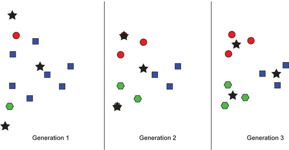
Conceptually, k-means is actually quite simple: In each iteration, every data point is associated with the cluster that it is closest to in terms of the cluster’s center. That center moves as new points are associated with the cluster. This is illustrated in figure 6.1.
Figure 6.1. An example of k-means running through three generations on an arbitrary data set. Stars indicate centroids. Colors and shapes represent current cluster membership (which changes).
We will implement a class for maintaining state and running the algorithm, similar to GeneticAlgorithm in chapter 5. We now return to the kmeans.py file.
Listing 6.3. kmeans.py continued
Point = TypeVar('Point', bound=DataPoint)

class KMeans(Generic[Point]):
    @dataclass
    class Cluster:
        points: List[Point]
        centroid: DataPoint
KMeans is a generic class. It works with DataPoint or any subclass of DataPoint, as defined by the Point type’s bound. It has an internal class, Cluster, that keeps track of the individual clusters in the operation. Each Cluster has data points and a centroid associated with it.
Now we will continue with the outer class’s __init__() method.
Listing 6.4. kmeans.py continued
def __init__(self, k: int, points: List[Point]) -> None:
    if k < 1: # k-means can't do negative or zero clusters
        raise ValueError("k must be >= 1")
    self._points: List[Point] = points
    self._zscore_normalize()
    # initialize empty clusters with random centroids
    self._clusters: List[KMeans.Cluster] = []
    for _ in range(k):
        rand_point: DataPoint = self._random_point()
        cluster: KMeans.Cluster = KMeans.Cluster([], rand_point)
        self._clusters.append(cluster)

@property
def _centroids(self) -> List[DataPoint]:
    return [x.centroid for x in self._clusters]
KMeans has an array, _points, associated with it. This is all of the points in the data set. The points are further divided between the clusters, which are stored in the appropriately titled _clusters variable. When KMeans is instantiated, it needs to know how many clusters to create (k). Every cluster initially has a random centroid. All of the data points that will be used in the algorithm are normalized by z-score. The computed _centroids property returns all of the centroids associated with the clusters that are associated with the algorithm.
Listing 6.5. kmeans.py continued
def _dimension_slice(self, dimension: int) -> List[float]:
    return [x.dimensions[dimension] for x in self._points]
_dimension_slice() is a convenience method that can be thought of as returning a column of data. It will return a list composed of every value at a particular index in every data point. For instance, if the data points were of type DataPoint, then _dimension_ slice(0) would return a list of the value of the first dimension of every data point. This is helpful in the following normalization method.
Listing 6.6. kmeans.py continued
def _zscore_normalize(self) -> None:
    zscored: List[List[float]] = [[] for _ in range(len(self._points))]
    for dimension in range(self._points[0].num_dimensions):
        dimension_slice: List[float] = self._dimension_slice(dimension)
        for index, zscore in enumerate(zscores(dimension_slice)):
            zscored[index].append(zscore)
    for i in range(len(self._points)):
        self._points[i].dimensions = tuple(zscored[i])
_zscore_normalize() replaces the values in the dimensions tuple of every data point with its z-scored equivalent. This uses the zscores() function that we defined for sequences of float earlier. Although the values in the dimensions tuple are replaced, the _originals tuple in the DataPoint are not. This is useful; the user of the algorithm can still retrieve the original values of the dimensions before normalization after the algorithm runs if they are stored in both places.
Listing 6.7. kmeans.py continued
def _random_point(self) -> DataPoint:
    rand_dimensions: List[float] = []
    for dimension in range(self._points[0].num_dimensions):
        values: List[float] = self._dimension_slice(dimension)
        rand_value: float = uniform(min(values), max(values))
        rand_dimensions.append(rand_value)
    return DataPoint(rand_dimensions)
The preceding _random_point() method is used in the __init__() method to create the initial random centroids for each cluster. It constrains the random values of each point to be within the range of the existing data points’ values. It uses the constructor we specified earlier on DataPoint to create a new point from an iterable of values.
Now we will look to our method for finding the appropriate cluster for a data point to belong to.
Listing 6.8. kmeans.py continued
# Find the closest cluster centroid to each point and assign the point to
     that cluster
def _assign_clusters(self) -> None:
    for point in self._points:
        closest: DataPoint = min(self._centroids,
    key=partial(DataPoint.distance, point))
        idx: int = self._centroids.index(closest)
        cluster: KMeans.Cluster = self._clusters[idx]
        cluster.points.append(point)
Throughout the book, we have created several functions that find the minimum or find the maximum in a list. This one is not dissimilar. In this case we are looking for the cluster centroid that has the minimum distance to each individual point. The point is then assigned to that cluster. The only tricky bit is the use of a function mediated by partial() as a key for min(). partial() takes a function and provides it with some of its parameters before the function is applied. In this case, we supply the DataPoint.distance() method with the point we are calculating from as its other parameter. This will result in each centroid’s distance to the point being computed and the lowest-distance centroid’s being returned by min().
Listing 6.9. kmeans.py continued
# Find the center of each cluster and move the centroid to there
def _generate_centroids(self) -> None:
    for cluster in self._clusters:
        if len(cluster.points) == 0: # keep the same centroid if no points
            continue
        means: List[float] = []
        for dimension in range(cluster.points[0].num_dimensions):
            dimension_slice: List[float] = [p.dimensions[dimension] for p in
      cluster.points]
            means.append(mean(dimension_slice))
        cluster.centroid = DataPoint(means)
After every point is assigned to a cluster, the new centroids are calculated. This involves calculating the mean of each dimension of every point in the cluster. The means of each dimension are then combined to find the “mean point” in the cluster, which becomes the new centroid. Note that we cannot use _dimension_slice() here, because the points in question are a subset of all of the points (just those belonging to a particular cluster). How could _dimension_slice() be rewritten to be more generic?
Now let’s look at the method that will actually execute the algorithm.
Listing 6.10. kmeans.py continued
def run(self, max_iterations: int = 100) -> List[KMeans.Cluster]:
    for iteration in range(max_iterations):
        for cluster in self._clusters: # clear all clusters
            cluster.points.clear()
        self._assign_clusters() # find cluster each point is closest to
        old_centroids: List[DataPoint] = deepcopy(self._centroids) # record
        self._generate_centroids() # find new centroids
        if old_centroids == self._centroids: # have centroids moved?
            print(f"Converged after {iteration} iterations")
            return self._clusters
    return self._clusters
run() is the purest expression of the original algorithm. The only change to the algorithm you may find unexpected is the removal of all points at the beginning of each iteration. If this were not to occur, the _assign_clusters() method, as written, would end up putting duplicate points in each cluster.
You can perform a quick test using test DataPoints and k set to 2.
Listing 6.11. kmeans.py continued
if __name__ == "__main__":
    point1: DataPoint = DataPoint([2.0, 1.0, 1.0])
    point2: DataPoint = DataPoint([2.0, 2.0, 5.0])
    point3: DataPoint = DataPoint([3.0, 1.5, 2.5])
    kmeans_test: KMeans[DataPoint] = KMeans(2, [point1, point2, point3])
    test_clusters: List[KMeans.Cluster] = kmeans_test.run()
    for index, cluster in enumerate(test_clusters):
        print(f"Cluster {index}: {cluster.points}")
Because there is randomness involved, your results may vary. The expected result is something along these lines:
Converged after 1 iterations
Cluster 0: [(2.0, 1.0, 1.0), (3.0, 1.5, 2.5)]
Cluster 1: [(2.0, 2.0, 5.0)]
6.3. Clustering governors by age and longitude
Every American state has a governor. In June 2017, those governors ranged in age from 42 to 79. If we take the United States from east to west, looking at each state by its longitude, perhaps we can find clusters of states with similar longitudes and similar-age governors. Figure 6.2 is a scatter plot of all 50 governors. The x-axis is state longitude, and the y-axis is governor age.
Figure 6.2. State governors, as of June 2017, plotted by state longitude and governor age
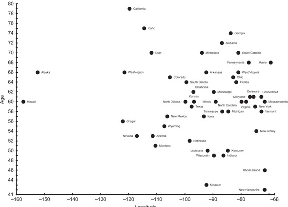
Are there any obvious clusters in figure 6.2? In this figure, the axes are not normalized. Instead, we are looking at raw data. If clusters were always obvious, there would be no need for clustering algorithms.
Let’s try running this data set through k-means. First, we will need a way of representing an individual data point.
Listing 6.12. governors.py
from __future__ import annotations
from typing import List
from data_point import DataPoint
from kmeans import KMeans

class Governor(DataPoint):
    def __init__(self, longitude: float, age: float, state: str) -> None:
        super().__init__([longitude, age])
        self.longitude = longitude
        self.age = age
        self.state = state

    def __repr__(self) -> str:
        return f"{self.state}: (longitude: {self.longitude}, age:
  {self.age})"
A Governor has two named and stored dimensions: longitude and age. Other than that, Governor makes no modifications to the machinery of its superclass, DataPoint, other than an overridden __repr__() for pretty printing. It would be pretty unreasonable to enter the following data manually, so check out the source code repository that accompanies this book.
Listing 6.13. governors.py continued
if __name__ == "__main__":
    governors: List[Governor] = [Governor(-86.79113, 72, "Alabama"),
     Governor(-152.404419, 66, "Alaska"),
                 Governor(-111.431221, 53, "Arizona"), Governor(-92.373123,
     66, "Arkansas"),
                 Governor(-119.681564, 79, "California"), Governor(-
     105.311104, 65, "Colorado"),
                 Governor(-72.755371, 61, "Connecticut"), Governor(-
     75.507141, 61, "Delaware"),
                 Governor(-81.686783, 64, "Florida"), Governor(-83.643074,
     74, "Georgia"),
                 Governor(-157.498337, 60, "Hawaii"), Governor(-114.478828,
     75, "Idaho"),
                 Governor(-88.986137, 60, "Illinois"), Governor(-86.258278,
     49, "Indiana"),
                 Governor(-93.210526, 57, "Iowa"), Governor(-96.726486, 60,
     "Kansas"),
                 Governor(-84.670067, 50, "Kentucky"), Governor(-91.867805,
     50, "Louisiana"),
                 Governor(-69.381927, 68, "Maine"), Governor(-76.802101, 61,
     "Maryland"),
                 Governor(-71.530106, 60, "Massachusetts"), Governor(-
     84.536095, 58, "Michigan"),
                 Governor(-93.900192, 70, "Minnesota"), Governor(-89.678696,
     62, "Mississippi"),
                 Governor(-92.288368, 43, "Missouri"), Governor(-110.454353,
     51, "Montana"),
                 Governor(-98.268082, 52, "Nebraska"), Governor(-117.055374,
     53, "Nevada"),
                 Governor(-71.563896, 42, "New Hampshire"), Governor(-
     74.521011, 54, "New Jersey"),
                 Governor(-106.248482, 57, "New Mexico"), Governor(-
     74.948051, 59, "New York"),
                 Governor(-79.806419, 60, "North Carolina"), Governor(-
     99.784012, 60, "North Dakota"),
                 Governor(-82.764915, 65, "Ohio"), Governor(-96.928917, 62,
     "Oklahoma"),
                 Governor(-122.070938, 56, "Oregon"), Governor(-77.209755,
     68, "Pennsylvania"),
                 Governor(-71.51178, 46, "Rhode Island"), Governor(-
     80.945007, 70, "South Carolina"),
                 Governor(-99.438828, 64, "South Dakota"), Governor(-
     86.692345, 58, "Tennessee"),
                 Governor(-97.563461, 59, "Texas"), Governor(-111.862434, 70,
     "Utah"),
                 Governor(-72.710686, 58, "Vermont"), Governor(-78.169968,
     60, "Virginia"),
                 Governor(-121.490494, 66, "Washington"), Governor(-
     80.954453, 66, "West Virginia"),
                 Governor(-89.616508, 49, "Wisconsin"), Governor(-107.30249,
     55, "Wyoming")]
We will run k-means with k set to 2.
Listing 6.14. governors.py continued
kmeans: KMeans[Governor] = KMeans(2, governors)
gov_clusters: List[KMeans.Cluster] = kmeans.run()
for index, cluster in enumerate(gov_clusters):
    print(f"Cluster {index}: {cluster.points}\n")
Because it starts with randomized centroids, every run of KMeans may potentially return different clusters. It takes some human analysis to see if the clusters are actually relevant. The following result is from a run that did have an interesting cluster:
Converged after 5 iterations
Cluster 0: [Alabama: (longitude: -86.79113, age: 72), Arizona: (longitude: -
     111.431221, age: 53), Arkansas: (longitude: -92.373123, age: 66),
     Colorado: (longitude: -105.311104, age: 65), Connecticut: (longitude: -
     72.755371, age: 61), Delaware: (longitude: -75.507141, age: 61),
     Florida: (longitude: -81.686783, age: 64), Georgia: (longitude: -
     83.643074, age: 74), Illinois: (longitude: -88.986137, age: 60),
     Indiana: (longitude: -86.258278, age: 49), Iowa: (longitude: -93.210526,
     age: 57), Kansas: (longitude: -96.726486, age: 60), Kentucky:
     (longitude: -84.670067, age: 50), Louisiana: (longitude: -91.867805,
     age: 50), Maine: (longitude: -69.381927, age: 68), Maryland: (longitude:
     -76.802101, age: 61), Massachusetts: (longitude: -71.530106, age: 60),
     Michigan: (longitude: -84.536095, age: 58), Minnesota: (longitude: -
     93.900192, age: 70), Mississippi: (longitude: -89.678696, age: 62),
     Missouri: (longitude: -92.288368, age: 43), Montana: (longitude: -
     110.454353, age: 51), Nebraska: (longitude: -98.268082, age: 52),
     Nevada: (longitude: -117.055374, age: 53), New Hampshire: (longitude: -
     71.563896, age: 42), New Jersey: (longitude: -74.521011, age: 54), New
     Mexico: (longitude: -106.248482, age: 57), New York: (longitude: -
     74.948051, age: 59), North Carolina: (longitude: -79.806419, age: 60),
     North Dakota: (longitude: -99.784012, age: 60), Ohio: (longitude: -
     82.764915, age: 65), Oklahoma: (longitude: -96.928917, age: 62),
     Pennsylvania: (longitude: -77.209755, age: 68), Rhode Island:
     (longitude: -71.51178, age: 46), South Carolina: (longitude: -80.945007,
     age: 70), South Dakota: (longitude: -99.438828, age: 64), Tennessee:
     (longitude: -86.692345, age: 58), Texas: (longitude: -97.563461, age:
     59), Vermont: (longitude: -72.710686, age: 58), Virginia: (longitude: -
     78.169968, age: 60), West Virginia: (longitude: -80.954453, age: 66),
     Wisconsin: (longitude: -89.616508, age: 49), Wyoming: (longitude: -
     107.30249, age: 55)]
Cluster 1: [Alaska: (longitude: -152.404419, age: 66), California:
     (longitude: -119.681564, age: 79), Hawaii: (longitude: -157.498337, age:
     60), Idaho: (longitude: -114.478828, age: 75), Oregon: (longitude: -
     122.070938, age: 56), Utah: (longitude: -111.862434, age: 70),
     Washington: (longitude: -121.490494, age: 66)]
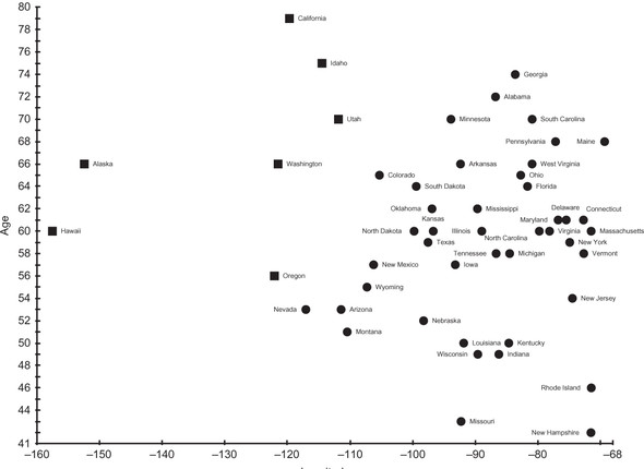
Cluster 1 represents the extreme Western states, all geographically next to each other (if you consider Alaska and Hawaii next to the Pacific coast states). They all have relatively old governors and hence formed an interesting cluster. Do folks on the Pacific Rim like older governors? We cannot determine anything conclusive from these clusters beyond a correlation. Figure 6.3 illustrates the result. Squares are cluster 1, and circles are cluster 0.
Figure 6.3. Data points in cluster 0 are designated by circles, and data points in cluster 1 are designated by squares.
Tip
It cannot be emphasized enough that your results with k-means using random initialization of centroids will vary. Be sure to run k-means multiple times with any data set.
6.4. Clustering Michael Jackson albums by length
Michael Jackson released 10 solo studio albums. In the following example, we will cluster those albums by looking at two dimensions: album length (in minutes) and number of tracks. This example is a nice contrast with the preceding governors example because it is easy to see the clusters in the original data set without even running k-means. An example like this can be a good way of debugging an implementation of a clustering algorithm.
Note
Both of the examples in this chapter make use of two-dimensional data points, but k-means can work with data points of any number of dimensions.
The example is presented here in its entirety as one code listing. If you look at the album data in the following code listing before even running the example, it is clear that Michael Jackson made longer albums toward the end of his career. So the two clusters of albums should probably be divided between earlier albums and later albums. HIStory: Past, Present, and Future, Book I is an outlier and can also logically end up in its own solo cluster. An outlier is a data point that lies outside the normal limits of a data set.
Listing 6.15. mj.py
from __future__ import annotations
from typing import List
from data_point import DataPoint
from kmeans import KMeans

class Album(DataPoint):
    def __init__(self, name: str, year: int, length: float, tracks: float) ->
     None:
        super().__init__([length, tracks])
        self.name = name
        self.year = year
        self.length = length
        self.tracks = tracks

    def __repr__(self) -> str:
        return f"{self.name}, {self.year}"

if __name__ == "__main__":
    albums: List[Album] = [Album("Got to Be There", 1972, 35.45, 10),
     Album("Ben", 1972, 31.31, 10),
                           Album("Music & Me", 1973, 32.09, 10),
     Album("Forever, Michael", 1975, 33.36, 10),
                           Album("Off the Wall", 1979, 42.28, 10),
     Album("Thriller", 1982, 42.19, 9),
                           Album("Bad", 1987, 48.16, 10), Album("Dangerous",
     1991, 77.03, 14),
                           Album("HIStory: Past, Present and Future, Book I",
     1995, 148.58, 30), Album("Invincible", 2001, 77.05, 16)]
    kmeans: KMeans[Album] = KMeans(2, albums)
    clusters: List[KMeans.Cluster] = kmeans.run()
    for index, cluster in enumerate(clusters):
        print(f"Cluster {index} Avg Length {cluster.centroid.dimensions[0]}
      Avg Tracks {cluster.centroid.dimensions[1]}: {cluster.points}\n")
Note that the attributes name and year are only recorded for labeling purposes and are not included in the actual clustering. Here is an example output:
Converged after 1 iterations
Cluster 0 Avg Length -0.5458820039179509 Avg Tracks -0.5009878988684237: [Got
     to Be There, 1972, Ben, 1972, Music & Me, 1973, Forever, Michael, 1975,
     Off the Wall, 1979, Thriller, 1982, Bad, 1987]

Cluster 1 Avg Length 1.2737246758085523 Avg Tracks 1.1689717640263217:
     [Dangerous, 1991, HIStory: Past, Present and Future, Book I, 1995,
     Invincible, 2001]
The reported cluster averages are interesting. Note that the averages are z-scores. Cluster 1’s three albums, Michael Jackson’s final three albums, were about one standard deviation longer than the average of all ten of his solo albums.
6.5. K-means clustering problems and extensions
When k-means clustering is implemented using random starting points, it may completely miss useful points of division within the data. This often results in a lot of trial and error for the operator. Figuring out the right value for “k” (the number of clusters) is also difficult and error prone if the operator does not have good insight into how many groups of data should exist.
There are more sophisticated versions of k-means that can try to make educated guesses or do automatic trial and error regarding these problematic variables. One popular variant is k-means++, which attempts to solve the initialization problem by choosing centroids based on a probability distribution of distance to every point instead of pure randomness. An even better option for many applications is to choose good starting regions for each of the centroids based on information about the data that is known ahead of time—in other words, a version of k-means where the user of the algorithm chooses the initial centroids.
The runtime for k-means clustering is proportional to the number of data points, the number of clusters, and the number of dimensions of the data points. It can become unusable in its basic form when there are a high number of points that have a large number of dimensions. There are extensions that try to not do as much calculation between every point and every center by evaluating whether a point really has the potential to move to another cluster before doing the calculation. Another option for numerous-point or high-dimension data sets is to run just a sampling of the data points through k-means. This will approximate the clusters that the full k-means algorithm may find.
Outliers in a data set may result in strange results for k-means. If an initial centroid happens to fall near an outlier, it could form a cluster of one (as could potentially happen with the HIStory album in the Michael Jackson example). K-means may run better with outliers removed.
Finally, the mean is not always considered a good measure of the center. K-medians looks at the median of each dimension, and k-medoids uses an actual point in the data set as the middle of each cluster. There are statistical reasons beyond the scope of this book for choosing each of these centering methods, but common sense dictates that for a tricky problem it may be worth trying each of them and sampling the results. The implementations of each are not that different.
6.6. Real-world applications
Clustering is often the purview of data scientists and statistical analysts. It is used widely as a way to interpret data in a variety of fields. K-means clustering, in particular, is a useful technique when little is known about the structure of the data set.
In data analysis, clustering is an essential technique. Imagine a police department that wants to know where to put cops on patrol. Imagine a fast-food franchise that wants to figure out where its best customers are, to send promotions. Imagine a boat-rental operator that wants to minimize accidents by analyzing when they occur and who causes them. Now imagine how they could solve their problems using clustering.
Clustering helps with pattern recognition. A clustering algorithm may detect a pattern that the human eye misses. For instance, clustering is sometimes used in biology to identify groups of incongruous cells.
In image recognition, clustering helps to identify nonobvious features. Individual pixels can be treated as data points with their relationship to one another being defined by distance and color difference.
In political science, clustering is sometimes used to find voters to target. Can a political party find disenfranchised voters concentrated in a single district that they should focus their campaign dollars on? What issues are similar voters likely to be concerned about?
6.7. Exercises
- Create a function that can import data from a CSV file into DataPoints.
- Create a function using an external library like matplotlib that creates a color-coded scatter plot of the results of any run of KMeans on a two-dimensional data set.
- Create a new initializer for KMeans that takes initial centroid positions instead of assigning them randomly.
- Research and implement the k-means++ algorithm.