Chapter 5. Genetic algorithms
Genetic algorithms are not used for everyday programmatic problems. They are called upon when traditional algorithmic approaches are insufficient for arriving at a solution to a problem in a reasonable amount of time. In other words, genetic algorithms are usually reserved for complex problems without easy solutions. If you need a sense of what some of these complex problems might be, feel free to read ahead in section 5.7 before proceeding. One interesting example, though, is protein-ligand docking and drug design. Computational biologists need to design molecules that will bind to receptors to deliver drugs. There may be no obvious algorithm for designing a particular molecule, but as you will see, sometimes genetic algorithms can provide an answer without much direction beyond a definition of the goal of a problem.
5.1. Biological background
In biology, the theory of evolution is an explanation of how genetic mutation, coupled with the constraints of an environment, leads to changes in organisms over time (including speciation—the creation of new species). The mechanism by which the well-adapted organisms succeed and the less well-adapted organisms fail is known as natural selection. Each generation of a species will include individuals with different (and sometimes new) traits that come about through genetic mutation. All individuals compete for limited resources to survive, and because there are more individuals than there are resources, some individuals must die.
An individual with a mutation that makes it better adapted for survival in its environment will have a higher probability of living and reproducing. Over time, the better-adapted individuals in an environment will have more children and through inheritance will pass on their mutations to those children. Therefore, a mutation that benefits survival is likely to eventually proliferate amongst a population.
For example, if bacteria are being killed by a specific antibiotic, and one individual bacterium in the population has a mutation in a gene that makes it more resistant to the antibiotic, it is more likely to survive and reproduce. If the antibiotic is continually applied over time, the children who have inherited the gene for antibiotic resistance will also be more likely to reproduce and have children of their own. Eventually the whole population may gain the mutation, as continued assault by the antibiotic kills off the individuals without the mutation. The antibiotic does not cause the mutation to develop, but it does lead to the proliferation of individuals with the mutation.
Natural selection has been applied in spheres beyond biology. Social Darwinism is natural selection applied to the sphere of social theory. In computer science, genetic algorithms are a simulation of natural selection to solve computational challenges.
A genetic algorithm includes a population (group) of individuals known as chromosomes. The chromosomes, each composed of genes that specify their traits, are competing to solve some problem. How well a chromosome solves a problem is defined by a fitness function.
The genetic algorithm goes through generations. In each generation, the chromosomes that are more fit are more likely to be selected to reproduce. There is also a probability in each generation that two chromosomes will have their genes merged. This is known as crossover. And finally, there is the important possibility in each generation that a gene in a chromosome may mutate (randomly change).
After the fitness function of some individual in the population crosses some specified threshold, or the algorithm runs through some specified maximum number of generations, the best individual (the one that scored highest in the fitness function) is returned.
Genetic algorithms are not a good solution for all problems. They depend on three partially or fully stochastic (randomly determined) operations: selection, crossover, and mutation. Therefore, they may not find an optimal solution in a reasonable amount of time. For most problems, more deterministic algorithms exist with better guarantees. But there are problems for which no fast deterministic algorithm exists. In these cases, genetic algorithms are a good choice.
5.2. A generic genetic algorithm
Genetic algorithms are often highly specialized and tuned for a particular application. In this chapter, we will define a generic genetic algorithm that can be used with multiple problems while not being particularly well tuned for any of them. It will include some configurable options, but the goal is to show the algorithm’s fundamentals instead of its tunability.
We will start by defining an interface for the individuals that the generic algorithm can operate on. The abstract class Chromosome defines four essential features. A chromosome must be able to do the following:
- Determine its own fitness
- Create an instance with randomly selected genes (for use in filling the first generation)
- Implement crossover (combine itself with another of the same type to create children)—in other words, mix itself with another chromosome
- Mutate—make a small, fairly random change in itself
Here is the code for Chromosome, codifying these four needs.
Listing 5.1. chromosome.py
from __future__ import annotations
from typing import TypeVar, Tuple, Type
from abc import ABC, abstractmethod

T = TypeVar('T', bound='Chromosome') # for returning self

# Base class for all chromosomes; all methods must be overridden
class Chromosome(ABC):
    @abstractmethod
    def fitness(self) -> float:
        ...

    @classmethod
    @abstractmethod
    def random_instance(cls: Type[T]) -> T:
        ...

    @abstractmethod
    def crossover(self: T, other: T) -> Tuple[T, T]:
        ...

    @abstractmethod
    def mutate(self) -> None:
        ...
Tip
You’ll notice in its constructor that the TypeVar T is bound to Chromosome. This means that anything that fills in a variable that is of type T must be an instance of a Chromosome or a subclass of Chromosome.
We will implement the algorithm itself (the code that will manipulate chromosomes) as a generic class that is open to subclassing for future specialized applications. Before we do so, though, let’s revisit the description of a genetic algorithm from the beginning of the chapter and clearly define the steps that a genetic algorithm takes:
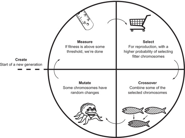
- Create an initial population of random chromosomes for the first generation of the algorithm.
- Measure the fitness of each chromosome in this generation of the population. If any exceeds the threshold, return it, and the algorithm ends.
- Select some individuals to reproduce, with a higher probability of selecting those with the highest fitness.
- Crossover (combine), with some probability, some of the selected chromosomes to create children that represent the population of the next generation.
- Mutate, usually with a low probability, some of those chromosomes. The population of the new generation is now complete, and it replaces the population of the last generation.
- Return to step 2 unless the maximum number of generations has been reached. If that is the case, return the best chromosome found so far.
This general outline of a genetic algorithm (illustrated in figure 5.1) is missing a lot of important details. How many chromosomes should be in the population? What is the threshold that stops the algorithm? How should the chromosomes be selected for reproduction? How should they be combined (crossover) and at what probability? At what probability should mutations occur? How many generations should be run?
Figure 5.1. The general outline of a genetic algorithm
All of these points will be configurable in our GeneticAlgorithm class. We will define it piece by piece so we can talk about each piece separately.
Listing 5.2. genetic_algorithm.py
from __future__ import annotations
from typing import TypeVar, Generic, List, Tuple, Callable
from enum import Enum
from random import choices, random
from heapq import nlargest
from statistics import mean
from chromosome import Chromosome

C = TypeVar('C', bound=Chromosome) # type of the chromosomes


class GeneticAlgorithm(Generic[C]):
    SelectionType = Enum("SelectionType", "ROULETTE TOURNAMENT")
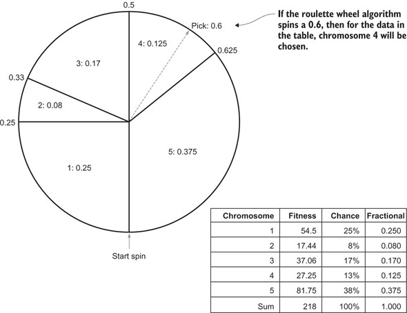
GeneticAlgorithm takes a generic type that conforms to Chromosome, and its name is C. The enum SelectionType is an internal type used for specifying the selection method used by the algorithm. The two most common genetic algorithm selection methods are known as roulette-wheel selection (sometimes called fitness proportionate selection) and tournament selection. The former gives every chromosome a chance of being picked, proportionate to its fitness. In tournament selection, a certain number of random chromosomes are challenged against one another, and the one with the best fitness is selected.
Listing 5.3. genetic_algorithm.py continued
def __init__(self, initial_population: List[C], threshold: float, max_
     generations: int = 100, mutation_chance: float = 0.01, crossover_chance:
     float = 0.7, selection_type: SelectionType = SelectionType.TOURNAMENT) -
     > None:
    self._population: List[C] = initial_population
    self._threshold: float = threshold
    self._max_generations: int = max_generations
    self._mutation_chance: float = mutation_chance
    self._crossover_chance: float = crossover_chance
    self._selection_type: GeneticAlgorithm.SelectionType = selection_type
    self._fitness_key: Callable = type(self._population[0]).fitness
The preceding are all properties of the genetic algorithm that will be configured at the time of creation, through __init__(). initial_population is the chromosomes in the first generation of the algorithm. threshold is the fitness level that indicates that a solution has been found for the problem that the genetic algorithm is trying to solve. max_generations is the maximum number of generations to run. If we have run that many generations and no solution with a fitness level beyond threshold has been found, the best solution that has been found will be returned. mutation_chance is the probability of each chromosome in each generation mutating. crossover_chance is the probability that two parents selected to reproduce have children that are a mixture of their genes; otherwise, the children are just duplicates of the parents. Finally, selection_type is the type of selection method to use, as delineated by the enum SelectionType.
The preceding init method takes a long list of parameters, most of which have default values. They set up instance versions of the configurable properties we just discussed. In our examples, _population is initialized with a random set of chromosomes using the Chromosome class’s random_instance() class method. In other words, the first generation of chromosomes is just composed of random individuals. This is a point of potential optimization for a more sophisticated genetic algorithm. Instead of starting with purely random individuals, the first generation could contain individuals that are closer to the solution, through some knowledge of the problem. This is referred to as seeding.
_fitness_key is a reference to the method we will be using throughout Genetic-Algorithm for calculating the fitness of a chromosome. Recall that this class needs to work with any subclass of Chromosome. Therefore, _fitness_key will differ by subclass. To get to it, we use type() to refer to the specific subclass of Chromosome that we are finding the fitness of.
Now we will examine the two selection methods that our class supports.
Listing 5.4. genetic_algorithm.py continued
# Use the probability distribution wheel to pick 2 parents
# Note: will not work with negative fitness results
def _pick_roulette(self, wheel: List[float]) -> Tuple[C, C]:
    return tuple(choices(self._population, weights=wheel, k=2))
Roulette-wheel selection is based on each chromosome’s proportion of fitness to the sum of all fitnesses in a generation. The chromosomes with the highest fitness have a better chance of being picked. The values that represent each chromosome’s fitness are provided in the parameter wheel. The actual picking is conveniently done by the choices() function from the Python standard library’s random module. This function takes a list of things we want to pick from, an equal-length list containing weights for each item in the first list, and how many items we want to pick.
If we were to implement this ourselves, we could calculate percentages of total fitness for each item (proportional fitnesses) that are represented by floating-point values between 0 and 1. A random number (pick) between 0 and 1 could be used to figure out which chromosome to select. The algorithm would work by decreasing pick by each chromosome’s proportional fitness value sequentially. When pick crosses 0, that’s the chromosome to select.
Does it make sense to you why this process results in each chromosome’s being pickable by its proportion? If not, think about it with pencil and paper. Consider drawing a proportional roulette wheel, as in figure 5.2.
Figure 5.2. An example of roulette-wheel selection in action
The most basic form of tournament selection is simpler than roulette-wheel selection. Instead of figuring out proportions, we simply pick k chromosomes from the whole population at random. The two chromosomes with the best fitness out of the randomly selected bunch win.
Listing 5.5. genetic_algorithm.py continued
# Choose num_participants at random and take the best 2
def _pick_tournament(self, num_participants: int) -> Tuple[C, C]:
    participants: List[C] = choices(self._population, k=num_participants)
    return tuple(nlargest(2, participants, key=self._fitness_key))
The code for _pick_tournament() first uses choices() to randomly pick num_participants from _population. Then it uses the nlargest() function from the heapq module to find the two largest individuals by _fitness_key. What is the right number for num_participants? As with many parameters in a genetic algorithm, trial and error may be the best way to determine it. One thing to keep in mind is that a higher number of participants in the tournament leads to less diversity in the population, because chromosomes with poor fitness are more likely to be eliminated in matchups.[1] More sophisticated forms of tournament selection may pick individuals that are not the best, but second- or third-best, based on some kind of decreasing probability model.
Artem Sokolov and Darrell Whitley, “Unbiased Tournament Selection,” GECCO’05 (June 25–29, 2005, Washington, D.C., U.S.A.), http://mng.bz/S7l6.
These two methods, _pick_roulette() and _pick_tournament(), are used for selection, which occurs during reproduction. Reproduction is implemented in _reproduce_and_replace(), and it also takes care of ensuring that a new population of an equal number of chromosomes replaces the chromosomes in the last generation.
Listing 5.6. genetic_algorithm.py continued
# Replace the population with a new generation of individuals
def _reproduce_and_replace(self) -> None:
    new_population: List[C] = []
    # keep going until we've filled the new generation
    while len(new_population) < len(self._population):
        # pick the 2 parents
        if self._selection_type == GeneticAlgorithm.SelectionType.ROULETTE:
            parents: Tuple[C, C] = self._pick_roulette([x.fitness() for x in
     self._population])
        else:
            parents = self._pick_tournament(len(self._population) // 2)
        # potentially crossover the 2 parents
        if random() < self._crossover_chance:
            new_population.extend(parents[0].crossover(parents[1]))
        else:
            new_population.extend(parents)
    # if we had an odd number, we'll have 1 extra, so we remove it
    if len(new_population) > len(self._population):
        new_population.pop()
    self._population = new_population # replace reference
In _reproduce_and_replace(), the following steps occur in broad strokes:
- Two chromosomes, called parents, are selected for reproduction using one of the two selection methods. For tournament selection, we always run the tournament amongst half of the total population, but this too could be a configuration option.
- There is _crossover_chance that the two parents will be combined to produce two new chromosomes, in which case they are added to new_population. If there are no children, the two parents are just added to new_population.
- If new_population has as many chromosomes as _population, it replaces it. Otherwise, we return to step 1.
The method that implements mutation, _mutate(), is very simple, with the details of how to perform a mutation being left to individual chromosomes.
Listing 5.7. genetic_algorithm.py continued
# With _mutation_chance probability mutate each individual
def _mutate(self) -> None:
    for individual in self._population:
        if random() < self._mutation_chance:
            individual.mutate()
We now have all of the building blocks needed to run the genetic algorithm. run() coordinates the measurement, reproduction (which includes selection), and mutation steps that bring the population from one generation to another. It also keeps track of the best (fittest) chromosome found at any point in the search.
Listing 5.8. genetic_algorithm.py continued
# Run the genetic algorithm for max_generations iterations
# and return the best individual found
def run(self) -> C:
    best: C = max(self._population, key=self._fitness_key)
    for generation in range(self._max_generations):
        # early exit if we beat threshold
        if best.fitness() >= self._threshold:
            return best
        print(f"Generation {generation} Best {best.fitness()} Avg
     {mean(map(self._fitness_key, self._population))}")
        self._reproduce_and_replace()
        self._mutate()
        highest: C = max(self._population, key=self._fitness_key)
        if highest.fitness() > best.fitness():
            best = highest # found a new best
    return best # best we found in _max_generations
best keeps track of the best chromosome found so far. The main loop executes _max_generations times. If any chromosome exceeds threshold in fitness, it is returned, and the method ends. Otherwise, it calls _reproduce_and_replace() as well as _mutate() to create the next generation and run the loop again. If _max_generations is reached, the best chromosome found so far is returned.
5.3. A naive test
The generic genetic algorithm, GeneticAlgorithm, will work with any type that implements Chromosome. As a test, we will start by implementing a simple problem that can be easily solved using traditional methods. We will try to maximize the equation 6x – x2 + 4y – y2. In other words, what values for x and y in that equation will yield the largest number?
The maximizing values can be found, using calculus, by taking partial derivatives and setting each equal to zero. The result is x = 3 and y = 2. Can our genetic algorithm reach the same result without using calculus? Let’s dig in.
Listing 5.9. simple_equation.py
from __future__ import annotations
from typing import Tuple, List
from chromosome import Chromosome
from genetic_algorithm import GeneticAlgorithm
from random import randrange, random
from copy import deepcopy

class SimpleEquation(Chromosome):
    def __init__(self, x: int, y: int) -> None:
        self.x: int = x
        self.y: int = y

    def fitness(self) -> float: # 6x - x^2 + 4y - y^2
        return 6 * self.x - self.x * self.x + 4 * self.y - self.y * self.y
    @classmethod
    def random_instance(cls) -> SimpleEquation:
        return SimpleEquation(randrange(100), randrange(100))

    def crossover(self, other: SimpleEquation) -> Tuple[SimpleEquation,
     SimpleEquation]:
        child1: SimpleEquation = deepcopy(self)
        child2: SimpleEquation = deepcopy(other)
        child1.y = other.y
        child2.y = self.y
        return child1, child2

    def mutate(self) -> None:
        if random() > 0.5: # mutate x
            if random() > 0.5:
                self.x += 1
            else:
                self.x -= 1
        else: # otherwise mutate y
            if random() > 0.5:
                self.y += 1
            else:
                self.y -= 1

    def __str__(self) -> str:
        return f"X: {self.x} Y: {self.y} Fitness: {self.fitness()}"
SimpleEquation conforms to Chromosome, and true to its name, it does so as simply as possible. The genes of a SimpleEquation chromosome can be thought of as x and y. The method fitness() evaluates x and y using the equation 6x – x2 + 4y – y2. The higher the value, the more fit the individual chromosome is, according to Genetic-Algorithm. In the case of a random instance, x and y are initially set to be random integers between 0 and 100, so random_instance() does not need to do anything other than instantiate a new SimpleEquation with these values. To combine one Simple-Equation with another in crossover(), the y values of the two instances are simply swapped to create the two children. mutate() randomly increments or decrements x or y. And that is pretty much it.
Because SimpleEquation conforms to Chromosome, we can already plug it into GeneticAlgorithm.
Listing 5.10. simple_equation.py continued
if __name__ == "__main__":
    initial_population: List[SimpleEquation] = [SimpleEquation.random_
     instance() for _ in range(20)]
    ga: GeneticAlgorithm[SimpleEquation] = GeneticAlgorithm(initial_population=initial_
     population, threshold=13.0, max_generations = 100,
     mutation_chance = 0.1, crossover_chance = 0.7)
    result: SimpleEquation = ga.run()
    print(result)
The parameters used here were derived through guess-and-check. You can try others. threshold is set to 13.0 because we already know the correct answer. When x = 3 and y = 2, the equation evaluates to 13.
If you did not previously know the answer, you might want to see the best result that could be found in a certain number of generations. In that case, you would set threshold to some arbitrarily large number. Remember, because genetic algorithms are stochastic, every run will be different.
Here is some sample output from a run in which the genetic algorithm solved the equation in nine generations:
Generation 0 Best -349 Avg -6112.3
Generation 1 Best 4 Avg -1306.7
Generation 2 Best 9 Avg -288.25
Generation 3 Best 9 Avg -7.35
Generation 4 Best 12 Avg 7.25
Generation 5 Best 12 Avg 8.5
Generation 6 Best 12 Avg 9.65
Generation 7 Best 12 Avg 11.7
Generation 8 Best 12 Avg 11.6
X: 3 Y: 2 Fitness: 13
As you can see, it came to the proper solution derived earlier with calculus, x = 3 and y = 2. You may also note that almost every generation, it got closer to the right answer.
Take into consideration that the genetic algorithm took more computational power than other methods would have to find the solution. In the real world, such a simple maximization problem would not be a good use of a genetic algorithm. But its simple implementation at least suffices to prove that our genetic algorithm works.
5.4. SEND+MORE=MONEY revisited
In chapter 3, we solved the classic cryptarithmetic problem SEND+MORE=MONEY using a constraint-satisfaction framework. (For a refresher on what the problem is all about, look back to the description in chapter 3.) The problem can also be solved in a reasonable amount of time using a genetic algorithm.
One of the largest difficulties in formulating a problem for a genetic algorithm solution is determining how to represent it. A convenient representation for cryptarithmetic problems is to use list indices as digits.[2] Hence, to represent the 10 possible digits (0, 1, 2, 3, 4, 5, 6, 7, 8, 9), a 10-element list is required. The characters to be searched within the problem can then be shifted around from place to place. For example, if it is suspected that the solution to a problem includes the character “E” representing the digit 4, then list[4] = "E". SEND+MORE=MONEY has eight distinct letters (S, E, N, D, M, O, R, Y), leaving two slots in the array empty. They can be filled with spaces indicating no letter.
Reza Abbasian and Masoud Mazloom, “Solving Cryptarithmetic Problems Using Parallel Genetic Algorithm,” 2009 Second International Conference on Computer and Electrical Engineering, http://mng.bz/RQ7V.
A chromosome that represents the SEND+MORE=MONEY problem is represented in SendMoreMoney2. Note how the fitness() method is strikingly similar to satisfied() from SendMoreMoneyConstraint in chapter 3.
Listing 5.11. send_more_money2.py
from __future__ import annotations
from typing import Tuple, List
from chromosome import Chromosome
from genetic_algorithm import GeneticAlgorithm
from random import shuffle, sample
from copy import deepcopy

class SendMoreMoney2(Chromosome):
    def __init__(self, letters: List[str]) -> None:
        self.letters: List[str] = letters

    def fitness(self) -> float:
        s: int = self.letters.index("S")
        e: int = self.letters.index("E")
        n: int = self.letters.index("N")
        d: int = self.letters.index("D")
        m: int = self.letters.index("M")
        o: int = self.letters.index("O")
        r: int = self.letters.index("R")
        y: int = self.letters.index("Y")
        send: int = s * 1000 + e * 100 + n * 10 + d
        more: int = m * 1000 + o * 100 + r * 10 + e
        money: int = m * 10000 + o * 1000 + n * 100 + e * 10 + y
        difference: int = abs(money - (send + more))
        return 1 / (difference + 1)

    @classmethod
    def random_instance(cls) -> SendMoreMoney2:
        letters = ["S", "E", "N", "D", "M", "O", "R", "Y", " ", " "]
        shuffle(letters)
        return SendMoreMoney2(letters)

    def crossover(self, other: SendMoreMoney2) -> Tuple[SendMoreMoney2,
     SendMoreMoney2]:
        child1: SendMoreMoney2 = deepcopy(self)
        child2: SendMoreMoney2 = deepcopy(other)
        idx1, idx2 = sample(range(len(self.letters)), k=2)
        l1, l2 = child1.letters[idx1], child2.letters[idx2]
        child1.letters[child1.letters.index(l2)], child1.letters[idx2] =
     child1.letters[idx2], l2
        child2.letters[child2.letters.index(l1)], child2.letters[idx1] =
     child2.letters[idx1], l1
        return child1, child2

    def mutate(self) -> None: # swap two letters' locations
        idx1, idx2 = sample(range(len(self.letters)), k=2)
        self.letters[idx1], self.letters[idx2] = self.letters[idx2],
     self.letters[idx1]

    def __str__(self) -> str:
        s: int = self.letters.index("S")
        e: int = self.letters.index("E")
        n: int = self.letters.index("N")
        d: int = self.letters.index("D")
        m: int = self.letters.index("M")
        o: int = self.letters.index("O")
        r: int = self.letters.index("R")
        y: int = self.letters.index("Y")
        send: int = s * 1000 + e * 100 + n * 10 + d
        more: int = m * 1000 + o * 100 + r * 10 + e
        money: int = m * 10000 + o * 1000 + n * 100 + e * 10 + y
        difference: int = abs(money - (send + more))
        return f"{send} + {more} = {money} Difference: {difference}"
There is, however, a major difference between satisfied() in chapter 3 and fitness() here. Here, we return 1 / (difference + 1). difference is the absolute value of the difference between MONEY and SEND+MORE. This represents how far off the chromosome is from solving the problem. If we were trying to minimize the fitness(), returning difference on its own would be fine. But because Genetic-Algorithm tries to maximize the value of fitness(), it needs to be flipped (so smaller values look like larger values), and that is why 1 is divided by difference. 1 is added to difference first, so that a difference of 0 does not yield a fitness() of 0 but instead of 1. Table 5.1 illustrates how this works.
Table 5.1. How the equation 1 / (difference + 1) yields fitnesses for maximization
|
difference |
difference + 1 |
fitness (1/(difference + 1)) |
|---|---|---|
| 0 | 1 | 1 |
| 1 | 2 | 0.5 |
| 2 | 3 | 0.25 |
| 3 | 4 | 0.125 |
Remember, lower differences are better, and higher fitnesses are better. Because this formula causes those two facts to line up, it works well. Dividing 1 by a fitness value is a simple way to convert a minimization problem into a maximization problem. It does introduce some biases, though, so it is not foolproof.[3]
For example, we might end up with more numbers closer to 0 than we will closer to 1 if we were to simply divide 1 by a uniform distribution of integers, which—with the subtleties of how typical microprocessors interpret floating-point numbers—could lead to some unexpected results. An alternative way to convert a minimization problem into a maximization problem is to simply flip the sign (make it negative instead of positive). However, this will only work if the values are all positive to begin with.
random_instance() makes use of the shuffle() function in the random module. crossover() selects two random indices in the letters lists of both chromosomes and swaps letters so that we end up with one letter from the first chromosome in the same place in the second chromosome, and vice versa. It performs these swaps in children so that the placement of letters in the two children ends up being a combination of the parents. mutate() swaps two random locations in the letters list.
We can plug SendMoreMoney2 into GeneticAlgorithm just as easily as we plugged in SimpleEquation. But be forewarned: This is a fairly tough problem, and it will take a long time to execute if the parameters are not well tweaked. And there’s still some randomness even if one gets them right! The problem may be solved in a few seconds or a few minutes. Unfortunately, that is the nature of genetic algorithms.
Listing 5.12. send_more_money2.py continued
if __name__ == "__main__":
    initial_population: List[SendMoreMoney2] = [SendMoreMoney2.random_
     instance() for _ in range(1000)]
    ga: GeneticAlgorithm[SendMoreMoney2] = GeneticAlgorithm(initial_population=initial_
     population, threshold=1.0, max_generations = 1000,
     mutation_chance = 0.2, crossover_chance = 0.7, selection_
     type=GeneticAlgorithm.SelectionType.ROULETTE)
    result: SendMoreMoney2 = ga.run()
    print(result)
The following output is from a run that solved the problem in 3 generations using 1,000 individuals in each generation (as created above). See if you can mess around with the configurable parameters of GeneticAlgorithm and get a similar result with fewer individuals. Does it seem to work better with roulette selection than it does with tournament selection?
Generation 0 Best 0.0040650406504065045 Avg 8.854014252391551e-05
Generation 1 Best 0.16666666666666666 Avg 0.001277329479413134
Generation 2 Best 0.5 Avg 0.014920889170684687
8324 + 913 = 9237 Difference: 0
This solution indicates that SEND = 8324, MORE = 913, and MONEY = 9237. How is that possible? It looks like letters are missing from the solution. In fact, if M = 0, there are several solutions to the problem not possible in the version from chapter 3. MORE is actually 0913 here, and MONEY is 09237. The 0 is just ignored.
5.5. Optimizing list compression
Suppose that we have some information we want to compress. Suppose that it is a list of items, and we do not care about the order of the items, as long as all of them are intact. What order of the items will maximize the compression ratio? Did you even know that the order of the items will affect the compression ratio for most compression algorithms?
The answer will depend on the compression algorithm used. For this example, we will use the compress() function from the zlib module with its standard settings. The solution is shown here in its entirety for a list of 12 first names. If we do not run the genetic algorithm and we just run compress() on the 12 names in the order they were originally presented, the resulting compressed data will be 165 bytes.
Listing 5.13. list_compression.py
from __future__ import annotations
from typing import Tuple, List, Any
from chromosome import Chromosome
from genetic_algorithm import GeneticAlgorithm
from random import shuffle, sample
from copy import deepcopy
from zlib import compress
from sys import getsizeof
from pickle import dumps

# 165 bytes compressed
PEOPLE: List[str] = ["Michael", "Sarah", "Joshua", "Narine", "David",
     "Sajid", "Melanie", "Daniel", "Wei", "Dean", "Brian", "Murat", "Lisa"]


class ListCompression(Chromosome):
    def __init__(self, lst: List[Any]) -> None:
        self.lst: List[Any] = lst

    @property
    def bytes_compressed(self) -> int:
        return getsizeof(compress(dumps(self.lst)))

    def fitness(self) -> float:
        return 1 / self.bytes_compressed

    @classmethod
    def random_instance(cls) -> ListCompression:
        mylst: List[str] = deepcopy(PEOPLE)
        shuffle(mylst)
        return ListCompression(mylst)

    def crossover(self, other: ListCompression) -> Tuple[ListCompression,
     ListCompression]:
        child1: ListCompression = deepcopy(self)
        child2: ListCompression = deepcopy(other)
        idx1, idx2 = sample(range(len(self.lst)), k=2)
        l1, l2 = child1.lst[idx1], child2.lst[idx2]
        child1.lst[child1.lst.index(l2)], child1.lst[idx2] =
     child1.lst[idx2], l2
        child2.lst[child2.lst.index(l1)], child2.lst[idx1] =
     child2.lst[idx1], l1
        return child1, child2

    def mutate(self) -> None: # swap two locations
        idx1, idx2 = sample(range(len(self.lst)), k=2)
        self.lst[idx1], self.lst[idx2] = self.lst[idx2], self.lst[idx1]

    def __str__(self) -> str:
        return f"Order: {self.lst} Bytes: {self.bytes_compressed}"

if __name__ == "__main__":
    initial_population: List[ListCompression] = [ListCompression.random_
     instance() for _ in range(1000)]
    ga: GeneticAlgorithm[ListCompression] = GeneticAlgorithm(initial_population=initial_
     population, threshold=1.0, max_generations = 1000,
     mutation_chance = 0.2, crossover_chance = 0.7, selection_
     type=GeneticAlgorithm.SelectionType.TOURNAMENT)
    result: ListCompression = ga.run()
    print(result)
Note how similar this implementation is to the implementation from SEND+ MORE=MONEY in section 5.4. The crossover() and mutate() functions are essentially the same. In both problems’ solutions, we are taking a list of items and continually rearranging them and testing those rearrangements. One could write a generic superclass for both problems’ solutions that would work with a wide variety of problems. Any problem that can be represented as a list of items that needs to find its optimal order could be solved the same way. The only real point of customization for the subclasses would be their respective fitness functions.
If we run list_compression.py, it may take a very long time to complete. This is because we don’t know what constitutes the “right” answer ahead of time, unlike the prior two problems, so we have no real threshold that we are working toward. Instead, we set the number of generations and the number of individuals in each generation to an arbitrarily high number and hope for the best. What is the minimum number of bytes that rearranging the 12 names will yield in compression? Frankly, we don’t know the answer to that. In my best run, using the configuration in the preceding solution, after 546 generations, the genetic algorithm found an order of the 12 names that yielded 159 bytes compressed.
That’s only a savings of 6 bytes over the original order—a ~4% savings. One might say that 4% is irrelevant, but if this were a far larger list that would be transferred many times over the network, that could add up. Imagine if this were a 1 MB list that would eventually be transferred across the internet 10,000,000 times. If the genetic algorithm could optimize the order of the list for compression to save 4%, it would save ~40 kilobytes per transfer and ultimately 400 GB in bandwidth across all transfers. That’s not a huge amount, but perhaps it could be significant enough that it’s worth running the algorithm once to find a near optimal order for compression.
Consider this, though—we don’t really know if we found the optimal order for the 12 names, let alone for the hypothetical 1 MB list. How would we know if we did? Unless we have a deep understanding of the compression algorithm, we would have to try compressing every possible order of the list. Just for a list of 12 items, that’s a fairly unfeasible 479,001,600 possible orders (12!, where ! means factorial). Using a genetic algorithm that attempts to find optimality is perhaps more feasible, even if we don’t know whether its ultimate solution is truly optimal.
5.6. Challenges for genetic algorithms
Genetic algorithms are not a panacea. In fact, they are not suitable for most problems. For any problem in which a fast deterministic algorithm exists, a genetic algorithm approach does not make sense. Their inherently stochastic nature makes their runtimes unpredictable. To solve this problem, they can be cut off after a certain number of generations. But then it is not clear if a truly optimal solution has been found.
Steven Skiena, author of one of the most popular texts on algorithms, even went so far as to write this:
I have never encountered any problem where genetic algorithms seemed to me the right way to attack it. Further, I have never seen any computational results reported using genetic algorithms that have favorably impressed me.[4]
Steven Skiena, The Algorithm Design Manual, 2nd edition (Springer, 2009), p. 267.
Skiena’s view is a little extreme, but it is indicative of the fact that genetic algorithms should only be chosen when you are reasonably confident that a better solution does not exist. Another issue with genetic algorithms is determining how to represent a potential solution to a problem as a chromosome. The traditional practice is to represent most problems as binary strings (sequences of 1s and 0s, raw bits). This is often optimal in terms of space usage, and it lends itself to easy crossover functions. But most complex problems are not easily represented as divisible bit strings.
Another, more specific issue worth mentioning is challenges related to the roulette-wheel selection method described in this chapter. Roulette-wheel selection, sometimes referred to as fitness proportional selection, can lead to a lack of diversity in a population due to the dominance of relatively fit individuals each time selection is run. On the other hand, if fitness values are close together, roulette-wheel selection can lead to a lack of selection pressure.[5] Further, roulette-wheel selection, as constructed in this chapter, does not work for problems in which fitness can be measured with negative values, as in our simple equation example in section 5.3.
A.E. Eiben and J.E. Smith, Introduction to Evolutionary Computation, 2nd edition (Springer, 2015), p. 80.
In short, for most problems large enough to warrant using them, genetic algorithms cannot guarantee the discovery of an optimal solution in a predictable amount of time. For this reason, they are best utilized in situations that do not call for an optimal solution, but instead for a “good enough” solution. They are fairly easy to implement, but tweaking their configurable parameters can take a lot of trial and error.
5.7. Real-world applications
Despite what Skiena wrote, genetic algorithms are frequently and effectively applied in a myriad of problem spaces. They are often used on hard problems that do not require perfectly optimal solutions, such as constraint-satisfaction problems too large to be solved using traditional methods. One example is complex scheduling problems.
Genetic algorithms have found many applications in computational biology. They have been used successfully for protein-ligand docking, which is a search for the configuration of a small molecule when it is bound to a receptor. This is used in pharmaceutical research and to better understand mechanisms in nature.
The Traveling Salesman Problem, which we will revisit in chapter 9, is one of the most famous problems in computer science. A traveling salesman wants to find the shortest route on a map that visits every city exactly once and brings him back to his starting location. It may sound like minimum spanning trees in chapter 4, but it is different. In the Traveling Salesman, the solution is a giant cycle that minimizes the cost to traverse it, whereas a minimum spanning tree minimizes the cost to connect every city. A person traveling a minimum spanning tree of cities may have to visit the same city twice to reach every city. Even though they sound similar, there is no reasonably timed algorithm for finding a solution to the Traveling Salesman problem for an arbitrary number of cities. Genetic algorithms have been shown to find suboptimal, but pretty good, solutions in short periods of time. The problem is widely applicable to the efficient distribution of goods. For example, dispatchers of FedEx and UPS trucks use software to solve the Traveling Salesman problem every day. Algorithms that help solve the problem can cut costs in a large variety of industries.
In computer-generated art, genetic algorithms are sometimes used to mimic photographs using stochastic methods. Imagine 50 polygons placed randomly on a screen and gradually twisted, turned, moved, resized, and changed in color until they match a photograph as closely as possible. The result looks like the work of an abstract artist or, if more angular shapes are used, a stained-glass window.
Genetic algorithms are part of a larger field called evolutionary computation. One area of evolutionary computation closely related to genetic algorithms is genetic programming, in which programs use the selection, crossover, and mutation operations to modify themselves to find nonobvious solutions to programming problems. Genetic programming is not a widely used technique, but imagine a future where programs write themselves.
A benefit of genetic algorithms is that they lend themselves to easy parallelization. In the most obvious form, each population can be simulated on a separate processor. In the most granular form, each individual can be mutated and crossed, and have its fitness calculated in a separate thread. There are also many possibilities in between.
5.8. Exercises
- Add support to GeneticAlgorithm for an advanced form of tournament selection that may sometimes choose the second- or third-best chromosome, based on a diminishing probability.
- Add a new function to the constraint-satisfaction framework from chapter 3 that solves any arbitrary CSP using a genetic algorithm. A possible measure of fitness is the number of constraints that are resolved by a chromosome.
- Create a class, BitString, that implements Chromosome. Recall what a bit string is from chapter 1. Then use your new class to solve the simple equation problem from section 5.3. How can the problem be encoded as a bit string?