Chapter 4. Graph problems
A graph is an abstract mathematical construct that is used for modeling a real-world problem by dividing the problem into a set of connected nodes. We call each of the nodes a vertex and each of the connections an edge. For instance, a subway map can be thought of as a graph representing a transportation network. Each of the dots represents a station, and each of the lines represents a route between two stations. In graph terminology, we would call the stations “vertices” and the routes “edges.”
Why is this useful? Not only do graphs help us abstractly think about a problem, but they also let us apply several well-understood and performant search and optimization techniques. For instance, in the subway example, suppose we want to know the shortest route from one station to another. Or suppose we want to know the minimum amount of track needed to connect all of the stations. Graph algorithms that you will learn in this chapter can solve both of those problems. Further, graph algorithms can be applied to any kind of network problem—not just transportation networks. Think of computer networks, distribution networks, and utility networks. Search and optimization problems across all of these spaces can be solved using graph algorithms.
4.1. A map as a graph
In this chapter, we won’t work with a graph of subway stations, but instead cities of the United States and potential routes between them. Figure 4.1 is a map of the continental United States and the 15 largest metropolitan statistical areas (MSAs) in the country, as estimated by the U.S. Census Bureau.[1]
Data is from the United States Census Bureau’s American Fact Finder, https://factfinder.census.gov/.
Figure 4.1. A map of the 15 largest MSAs in the United States
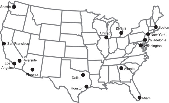
Famous entrepreneur Elon Musk has suggested building a new high-speed transportation network composed of capsules traveling in pressurized tubes. According to Musk, the capsules would travel at 700 miles per hour and be suitable for cost-effective transportation between cities less than 900 miles apart.[2] He calls this new transportation system the “Hyperloop.” In this chapter we will explore classic graph problems in the context of building out this transportation network.
Elon Musk, “Hyperloop Alpha,” http://mng.bz/chmu.
Musk initially proposed the Hyperloop idea for connecting Los Angeles and San Francisco. If one were to build a national Hyperloop network, it would make sense to do so between America’s largest metropolitan areas. In figure 4.2, the state outlines from figure 4.1 are removed. In addition, each of the MSAs is connected with some of its neighbors. To make the graph a little more interesting, those neighbors are not always the MSA’s closest neighbors.
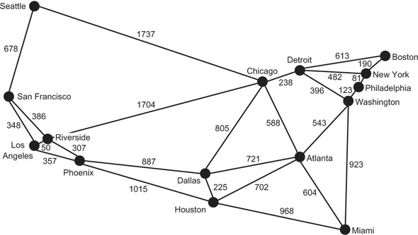
Figure 4.2 is a graph with vertices representing the 15 largest MSAs in the United States and edges representing potential Hyperloop routes between cities. The routes were chosen for illustrative purposes. Certainly, other potential routes could be part of a new Hyperloop network.
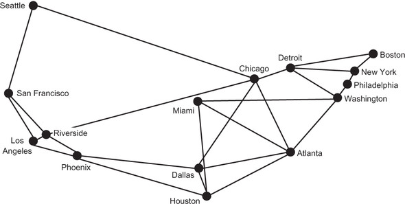
This abstract representation of a real-world problem highlights the power of graphs. With this abstraction, we can ignore the geography of the United States and concentrate on thinking about the potential Hyperloop network simply in the context of connecting cities. In fact, as long as we keep the edges the same, we can think about the problem with a different-looking graph. In figure 4.3, for example, the location of Miami has moved. The graph in figure 4.3, being an abstract representation, can address the same fundamental computational problems as the graph in figure 4.2, even if Miami is not where we would expect it. But for our sanity, we will stick with the representation in figure 4.2.
Figure 4.2. A graph with vertices representing the 15 largest MSAs in the United States and edges representing potential Hyperloop routes between them
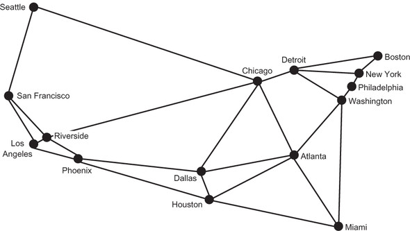
Figure 4.3. An equivalent graph to that in figure 4.2, with the location of Miami moved
4.2. Building a graph framework
Python can be programmed in many different styles. But at its heart, Python is an object-oriented programming language. In this section we will define two different types of graphs: unweighted and weighted. Weighted graphs, which we will discuss later in the chapter, associate a weight (read number, such as a length in the case of our example) with each edge.
We will make use of the inheritance model, fundamental to Python’s object-oriented class hierarchies, so we do not duplicate our effort. The weighted classes in our data model will be subclasses of their unweighted counterparts. This will allow them to inherit much of their functionality, with small tweaks for what makes a weighted graph distinct from an unweighted graph.
We want this graph framework to be as flexible as possible so that it can represent as many different problems as possible. To achieve this goal, we will use generics to abstract away the type of the vertices. Every vertex will ultimately be assigned an integer index, but it will be stored as the user-defined generic type.
Let’s start work on the framework by defining the Edge class, which is the simplest machinery in our graph framework.
Listing 4.1. edge.py
from __future__ import annotations
from dataclasses import dataclass


@dataclass
class Edge:
    u: int # the "from" vertex
    v: int # the "to" vertex

    def reversed(self) -> Edge:
        return Edge(self.v, self.u)

    def __str__(self) -> str:
        return f"{self.u} -> {self.v}"
An Edge is defined as a connection between two vertices, each of which is represented by an integer index. By convention, u is used to refer to the first vertex, and v is used to represent the second vertex. You can also think of u as “from” and v as “to.” In this chapter, we are only working with undirected graphs (graphs with edges that allow travel in both directions), but in directed graphs, also known as digraphs, edges can also be one-way. The reversed() method is meant to return an Edge that travels in the opposite direction of the edge it is applied to.
Note
The Edge class uses a new feature in Python 3.7: dataclasses. A class marked with the @dataclass decorator saves some tedium by automatically creating an __init__() method that instantiates instance variables for any variables declared with type annotations in the class’s body. Dataclasses can also automatically create other special methods for a class. Which special methods are automatically created is configurable via the decorator. See the Python documentation on dataclasses for details (https://docs.python.org/3/library/dataclasses.html). In short, a dataclass is a way of saving ourselves some typing.
The Graph class focuses on the essential role of a graph: associating vertices with edges. Again, we want to let the actual types of the vertices be whatever the user of the framework desires. This lets the framework be used for a wide range of problems without needing to make intermediate data structures that glue everything together. For example, in a graph like the one for Hyperloop routes, we might define the type of the vertices to be str, because we would use strings like “New York” and “Los Angeles” as the vertices. Let’s begin the Graph class.
Listing 4.2. graph.py
from typing import TypeVar, Generic, List, Optional
from edge import Edge

V = TypeVar('V') # type of the vertices in the graph


class Graph(Generic[V]):
    def __init__(self, vertices: List[V] = []) -> None:
        self._vertices: List[V] = vertices
        self._edges: List[List[Edge]] = [[] for _ in vertices]
The _vertices list is the heart of a Graph. Each vertex will be stored in the list, but we will later refer to them by their integer index in the list. The vertex itself may be a complex data type, but its index will always be an int, which is easy to work with. On another level, by putting this index between graph algorithms and the _vertices array, it allows us to have two vertices that are equal in the same graph. (Imagine a graph with a country’s cities as vertices, where the country has more than one city named “Springfield.”) Even though they are the same, they will have different integer indexes.
There are many ways to implement a graph data structure, but the two most common are to use a vertex matrix or adjacency lists. In a vertex matrix, each cell of the matrix represents the intersection of two vertices in the graph, and the value of that cell indicates the connection (or lack thereof) between them. Our graph data structure uses adjacency lists. In this graph representation, every vertex has a list of vertices that it is connected to. Our specific representation uses a list of lists of edges, so for every vertex there is a list of edges via which the vertex is connected to other vertices. _edges is this list of lists.
The rest of the Graph class is now presented in its entirety. You will notice the use of short, mostly one-line methods, with verbose and clear method names. This should make the rest of the class largely self-explanatory, but short comments are included so that there is no room for misinterpretation.
Listing 4.3. graph.py continued
@property
def vertex_count(self) -> int:
    return len(self._vertices) # Number of vertices

@property
def edge_count(self) -> int:
    return sum(map(len, self._edges)) # Number of edges

# Add a vertex to the graph and return its index
def add_vertex(self, vertex: V) -> int:
    self._vertices.append(vertex)
    self._edges.append([]) # Add empty list for containing edges
    return self.vertex_count - 1 # Return index of added vertex

# This is an undirected graph,
# so we always add edges in both directions
def add_edge(self, edge: Edge) -> None:
    self._edges[edge.u].append(edge)
    self._edges[edge.v].append(edge.reversed())

# Add an edge using vertex indices (convenience method)
def add_edge_by_indices(self, u: int, v: int) -> None:
    edge: Edge = Edge(u, v)
    self.add_edge(edge)

# Add an edge by looking up vertex indices (convenience method)
def add_edge_by_vertices(self, first: V, second: V) -> None:
    u: int = self._vertices.index(first)
    v: int = self._vertices.index(second)
    self.add_edge_by_indices(u, v)

# Find the vertex at a specific index
def vertex_at(self, index: int) -> V:
    return self._vertices[index]

# Find the index of a vertex in the graph
def index_of(self, vertex: V) -> int:
    return self._vertices.index(vertex)

# Find the vertices that a vertex at some index is connected to
def neighbors_for_index(self, index: int) -> List[V]:
    return list(map(self.vertex_at, [e.v for e in self._edges[index]]))

# Look up a vertice's index and find its neighbors (convenience method)
def neighbors_for_vertex(self, vertex: V) -> List[V]:
    return self.neighbors_for_index(self.index_of(vertex))

# Return all of the edges associated with a vertex at some index
def edges_for_index(self, index: int) -> List[Edge]:
    return self._edges[index]

# Look up the index of a vertex and return its edges (convenience method)
def edges_for_vertex(self, vertex: V) -> List[Edge]:
    return self.edges_for_index(self.index_of(vertex))

# Make it easy to pretty-print a Graph
def __str__(self) -> str:
    desc: str = ""
    for i in range(self.vertex_count):
        desc += f"{self.vertex_at(i)} -> {self.neighbors_for_index(i)}\n"
    return desc
Let’s step back for a moment and consider why this class has two versions of most of its methods. We know from the class definition that the list _vertices is a list of elements of type V, which can be any Python class. So we have vertices of type V that are stored in the _vertices list. But if we want to retrieve or manipulate them later, we need to know where they are stored in that list. Hence, every vertex has an index in the array (an integer) associated with it. If we don’t know a vertex’s index, we need to look it up by searching through _vertices. That is why there are two versions of every method. One operates on int indices, and one operates on V itself. The methods that operate on V look up the relevant indices and call the index-based function. Therefore, they can be considered convenience methods.
Most of the functions are fairly self-explanatory, but neighbors_for_index() deserves a little unpacking. It returns the neighbors of a vertex. A vertex’s neighbors are all of the other vertices that are directly connected to it by an edge. For example, in figure 4.2, New York and Washington are the only neighbors of Philadelphia. We find the neighbors for a vertex by looking at the ends (the vs) of all of the edges going out from it.
def neighbors_for_index(self, index: int) -> List[V]:
    return list(map(self.vertex_at, [e.v for e in self._edges[index]]))
_edges[index] is the adjacency list, the list of edges through which the vertex in question is connected to other vertices. In the list comprehension passed to the map() call, e represents one particular edge, and e.v represents the index of the neighbor that the edge is connected to. map() will return all of the vertices (as opposed to just their indices), because map() applies the vertex_at() method on every e.v.
Another important thing to note is the way add_edge() works. add_edge() first adds an edge to the adjacency list of the “from” vertex (u) and then adds a reversed version of the edge to the adjacency list of the “to” vertex (v). The second step is necessary because this graph is undirected. We want every edge to be added in both directions; that means that u will be a neighbor of v in the same way that v is a neighbor of u. You can think of an undirected graph as being “bidirectional” if it helps you remember that it means any edge can be traversed in either direction.
def add_edge(self, edge: Edge) -> None:
    self._edges[edge.u].append(edge)
    self._edges[edge.v].append(edge.reversed())
As was mentioned earlier, we are only dealing with undirected graphs in this chapter. Beyond being undirected or directed, graphs can also be unweighted or weighted. A weighted graph is one that has some comparable value, usually numeric, associated with each of its edges. We could think of the weights in our potential Hyperloop network as being the distances between the stations. For now, though, we will deal with an unweighted version of the graph. An unweighted edge is simply a connection between two vertices; hence, the Edge class is unweighted, and the Graph class is unweighted. Another way of putting it is that in an unweighted graph we know which vertices are connected, whereas in a weighted graph we know which vertices are connected and also know something about those connections.
4.2.1. Working with Edge and Graph
Now that we have concrete implementations of Edge and Graph, we can create a representation of the potential Hyperloop network. The vertices and edges in city_graph correspond to the vertices and edges represented in figure 4.2. Using generics, we can specify that vertices will be of type str (Graph[str]). In other words, the str type fills in for the type variable V.
Listing 4.4. graph.py continued
if __name__ == "__main__":
    # test basic Graph construction
    city_graph: Graph[str] = Graph(["Seattle", "San Francisco", "Los
     Angeles", "Riverside", "Phoenix", "Chicago", "Boston", "New York",
     "Atlanta", "Miami", "Dallas", "Houston", "Detroit", "Philadelphia",
     "Washington"])
    city_graph.add_edge_by_vertices("Seattle", "Chicago")
    city_graph.add_edge_by_vertices("Seattle", "San Francisco")
    city_graph.add_edge_by_vertices("San Francisco", "Riverside")
    city_graph.add_edge_by_vertices("San Francisco", "Los Angeles")
    city_graph.add_edge_by_vertices("Los Angeles", "Riverside")
    city_graph.add_edge_by_vertices("Los Angeles", "Phoenix")
    city_graph.add_edge_by_vertices("Riverside", "Phoenix")
    city_graph.add_edge_by_vertices("Riverside", "Chicago")
    city_graph.add_edge_by_vertices("Phoenix", "Dallas")
    city_graph.add_edge_by_vertices("Phoenix", "Houston")
    city_graph.add_edge_by_vertices("Dallas", "Chicago")
    city_graph.add_edge_by_vertices("Dallas", "Atlanta")
    city_graph.add_edge_by_vertices("Dallas", "Houston")
    city_graph.add_edge_by_vertices("Houston", "Atlanta")
    city_graph.add_edge_by_vertices("Houston", "Miami")
    city_graph.add_edge_by_vertices("Atlanta", "Chicago")
    city_graph.add_edge_by_vertices("Atlanta", "Washington")
    city_graph.add_edge_by_vertices("Atlanta", "Miami")
    city_graph.add_edge_by_vertices("Miami", "Washington")
    city_graph.add_edge_by_vertices("Chicago", "Detroit")
    city_graph.add_edge_by_vertices("Detroit", "Boston")
    city_graph.add_edge_by_vertices("Detroit", "Washington")
    city_graph.add_edge_by_vertices("Detroit", "New York")
    city_graph.add_edge_by_vertices("Boston", "New York")
    city_graph.add_edge_by_vertices("New York", "Philadelphia")
    city_graph.add_edge_by_vertices("Philadelphia", "Washington")
    print(city_graph)
city_graph has vertices of type str, and we indicate each vertex with the name of the MSA that it represents. It is irrelevant in what order we add the edges to city_graph. Because we implemented __str__() with a nicely printed description of the graph, we can now pretty-print (that’s a real term!) the graph. You should get output similar to the following:
Seattle -> ['Chicago', 'San Francisco']
San Francisco -> ['Seattle', 'Riverside', 'Los Angeles']
Los Angeles -> ['San Francisco', 'Riverside', 'Phoenix']
Riverside -> ['San Francisco', 'Los Angeles', 'Phoenix', 'Chicago']
Phoenix -> ['Los Angeles', 'Riverside', 'Dallas', 'Houston']
Chicago -> ['Seattle', 'Riverside', 'Dallas', 'Atlanta', 'Detroit']
Boston -> ['Detroit', 'New York']
New York -> ['Detroit', 'Boston', 'Philadelphia']
Atlanta -> ['Dallas', 'Houston', 'Chicago', 'Washington', 'Miami']
Miami -> ['Houston', 'Atlanta', 'Washington']
Dallas -> ['Phoenix', 'Chicago', 'Atlanta', 'Houston']
Houston -> ['Phoenix', 'Dallas', 'Atlanta', 'Miami']
Detroit -> ['Chicago', 'Boston', 'Washington', 'New York']
Philadelphia -> ['New York', 'Washington']
Washington -> ['Atlanta', 'Miami', 'Detroit', 'Philadelphia']
4.3. Finding the shortest path
The Hyperloop is so fast that for optimizing travel time from one station to another, it probably matters less how long the distances are between the stations and more how many hops it takes (how many stations need to be visited) to get from one station to another. Each station may involve a layover, so just like with flights, the fewer stops the better.
In graph theory, a set of edges that connects two vertices is known as a path. In other words, a path is a way of getting from one vertex to another vertex. In the context of the Hyperloop network, a set of tubes (edges) represents the path from one city (vertex) to another (vertex). Finding optimal paths between vertices is one of the most common problems that graphs are used for.
Informally, we can also think of a list of vertices sequentially connected to one another by edges as a path. This description is really just another side of the same coin. It is like taking a list of edges, figuring out which vertices they connect, keeping that list of vertices, and throwing away the edges. In this brief example, we will find such a list of vertices that connects two cities on our Hyperloop.
4.3.1. Revisiting breadth-first search (BFS)
In an unweighted graph, finding the shortest path means finding the path that has the fewest edges between the starting vertex and the destination vertex. To build out the Hyperloop network, it might make sense to first connect the furthest cities on the highly populated seaboards. That raises the question “What is the shortest path between Boston and Miami?”
TIP
This section assumes that you have read chapter 2. Before continuing, ensure that you are comfortable with the material on breadth-first search in chapter 2.
Luckily, we already have an algorithm for finding shortest paths, and we can reuse it to answer this question. Breadth-first search, introduced in chapter 2, is just as viable for graphs as it is for mazes. In fact, the mazes we worked with in chapter 2 really are graphs. The vertices are the locations in the maze, and the edges are the moves that can be made from one location to another. In an unweighted graph, a breadth-first search will find the shortest path between any two vertices.
We can reuse the breadth-first search implementation from chapter 2 and use it to work with Graph. In fact, we can reuse it completely unchanged. This is the power of writing code generically!
Recall that bfs() in chapter 2 requires three parameters: an initial state, a Callable (read function-like object) for testing for a goal, and a Callable that finds the successor states for a given state. The initial state will be the vertex represented by the string “Boston.” The goal test will be a lambda that checks if a vertex is equivalent to “Miami.” Finally, successor vertices can be generated by the Graph method neighbors_for_vertex().
With this plan in mind, we can add code to the end of the main section of graph.py to find the shortest route between Boston and Miami on city_graph.
Note
In listing 4.5, bfs, Node, and node_to_path are imported from the generic_search module in the Chapter2 package. To do this, the parent directory of graph.py is added to Python’s search path ('..'). This works because the code structure for the book’s repository has each chapter in its own directory, so our directory structure includes roughly Book->Chapter2-> generic_search.py and Book->Chapter4->graph.py. If your directory structure is significantly different, you will need to find a way to add generic_search.py to your path and possibly change the import statement. In a worst-case scenario, you can just copy generic_search.py to the same directory that contains graph.py and change the import statement to from generic_search import bfs, Node, node_to_path.
Listing 4.5. graph.py continued
# Reuse BFS from chapter 2 on city_graph
import sys
sys.path.insert(0, '..') # so we can access the Chapter2 package in the
     parent directory
from Chapter2.generic_search import bfs, Node, node_to_path

bfs_result: Optional[Node[V]] = bfs("Boston", lambda x: x == "Miami", city_
     graph.neighbors_for_vertex)
if bfs_result is None:
    print("No solution found using breadth-first search!")
else:
    path: List[V] = node_to_path(bfs_result)
    print("Path from Boston to Miami:")
    print(path)
The output should look something like this:
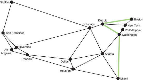
Path from Boston to Miami:
['Boston', 'Detroit', 'Washington', 'Miami']
Boston to Detroit to Washington to Miami, composed of three edges, is the shortest route between Boston and Miami in terms of the number of edges. Figure 4.4 highlights this route.
Figure 4.4. The shortest route between Boston and Miami, in terms of the number of edges, is highlighted.
4.4. Minimizing the cost of building the network
Imagine that we want to connect all 15 of the largest MSAs to the Hyperloop network. Our goal is to minimize the cost of rolling out the network, so that means using a minimum amount of track. Then the question is “How can we connect all of the MSAs using the minimum amount of track?”
4.4.1. Workings with weights
To understand the amount of track that a particular edge may require, we need to know the distance that the edge represents. This is an opportunity to re-introduce the concept of weights. In the Hyperloop network, the weight of an edge is the distance between the two MSAs that it connects. Figure 4.5 is the same as figure 4.2 except that it has a weight added to each edge, representing the distance in miles between the two vertices that the edge connects.
Figure 4.5. A weighted graph of the 15 largest MSAs in the United States, where each of the weights represents the distance between two MSAs in miles
To handle weights, we will need a subclass of Edge (WeightedEdge) and a subclass of Graph (WeightedGraph). Every WeightedEdge will have a float associated with it, representing its weight. Jarník’s algorithm, which we will cover shortly, requires the ability to compare one edge with another to determine the edge with the lowest weight. This is easy to do with numeric weights.
Listing 4.6. weighted_edge.py
from __future__ import annotations
from dataclasses import dataclass
from edge import Edge


@dataclass
class WeightedEdge(Edge):
    weight: float

    def reversed(self) -> WeightedEdge:
        return WeightedEdge(self.v, self.u, self.weight)

    # so that we can order edges by weight to find the minimum weight edge
    def __lt__(self, other: WeightedEdge) -> bool:
        return self.weight < other.weight

    def __str__(self) -> str:
        return f"{self.u} {self.weight}> {self.v}"
The implementation of WeightedEdge is not immensely different from that of Edge. It only differs in the addition of a weight property and the implementation of the < operator via __lt__(), so that two WeightedEdges are comparable. The < operator is only interested in looking at weights (as opposed to including the inherited properties u and v), because Jarník’s algorithm is interested in finding the smallest edge by weight.
A WeightedGraph inherits much of its functionality from Graph. Other than that, it has init methods; it has convenience methods for adding WeightedEdges; and it implements its own version of __str__(). There is also a new method, neighbors_for_index_with_weights(), that returns not only each neighbor, but also the weight of the edge that got to it. This method is useful for the new version of __str__().
Listing 4.7. weighted_graph.py
from typing import TypeVar, Generic, List, Tuple
from graph import Graph
from weighted_edge import WeightedEdge

V = TypeVar('V') # type of the vertices in the graph

class WeightedGraph(Generic[V], Graph[V]):
    def __init__(self, vertices: List[V] = []) -> None:
        self._vertices: List[V] = vertices
        self._edges: List[List[WeightedEdge]] = [[] for _ in vertices]

    def add_edge_by_indices(self, u: int, v: int, weight: float) -> None:
        edge: WeightedEdge = WeightedEdge(u, v, weight)
        self.add_edge(edge) # call superclass version

    def add_edge_by_vertices(self, first: V, second: V, weight: float) ->
     None:
        u: int = self._vertices.index(first)
        v: int = self._vertices.index(second)
        self.add_edge_by_indices(u, v, weight)

    def neighbors_for_index_with_weights(self, index: int) -> List[Tuple[V,
     float]]:
        distance_tuples: List[Tuple[V, float]] = []
        for edge in self.edges_for_index(index):
            distance_tuples.append((self.vertex_at(edge.v), edge.weight))
        return distance_tuples

    def __str__(self) -> str:
        desc: str = ""
        for i in range(self.vertex_count):
            desc += f"{self.vertex_at(i)} -> {self.neighbors_for_index_with_
    weights(i)}\n"
        return desc
It is now possible to actually define a weighted graph. The weighted graph we will work with is a representation of figure 4.5 called city_graph2.
Listing 4.8. weighted_graph.py continued
if __name__ == "__main__":
    city_graph2: WeightedGraph[str] = WeightedGraph(["Seattle", "San
     Francisco", "Los Angeles", "Riverside", "Phoenix", "Chicago", "Boston",
     "New York", "Atlanta", "Miami", "Dallas", "Houston", "Detroit",
     "Philadelphia", "Washington"])
    city_graph2.add_edge_by_vertices("Seattle", "Chicago", 1737)
    city_graph2.add_edge_by_vertices("Seattle", "San Francisco", 678)
    city_graph2.add_edge_by_vertices("San Francisco", "Riverside", 386)
    city_graph2.add_edge_by_vertices("San Francisco", "Los Angeles", 348)
    city_graph2.add_edge_by_vertices("Los Angeles", "Riverside", 50)
    city_graph2.add_edge_by_vertices("Los Angeles", "Phoenix", 357)
    city_graph2.add_edge_by_vertices("Riverside", "Phoenix", 307)
    city_graph2.add_edge_by_vertices("Riverside", "Chicago", 1704)
    city_graph2.add_edge_by_vertices("Phoenix", "Dallas", 887)
    city_graph2.add_edge_by_vertices("Phoenix", "Houston", 1015)
    city_graph2.add_edge_by_vertices("Dallas", "Chicago", 805)
    city_graph2.add_edge_by_vertices("Dallas", "Atlanta", 721)
    city_graph2.add_edge_by_vertices("Dallas", "Houston", 225)
    city_graph2.add_edge_by_vertices("Houston", "Atlanta", 702)
    city_graph2.add_edge_by_vertices("Houston", "Miami", 968)
    city_graph2.add_edge_by_vertices("Atlanta", "Chicago", 588)
    city_graph2.add_edge_by_vertices("Atlanta", "Washington", 543)
    city_graph2.add_edge_by_vertices("Atlanta", "Miami", 604)
    city_graph2.add_edge_by_vertices("Miami", "Washington", 923)
    city_graph2.add_edge_by_vertices("Chicago", "Detroit", 238)
    city_graph2.add_edge_by_vertices("Detroit", "Boston", 613)
    city_graph2.add_edge_by_vertices("Detroit", "Washington", 396)
    city_graph2.add_edge_by_vertices("Detroit", "New York", 482)
    city_graph2.add_edge_by_vertices("Boston", "New York", 190)
    city_graph2.add_edge_by_vertices("New York", "Philadelphia", 81)
    city_graph2.add_edge_by_vertices("Philadelphia", "Washington", 123)

    print(city_graph2)
Because WeightedGraph implements __str__(), we can pretty-print city_graph2. In the output, you will see both the vertices that each vertex is connected to and the weights of those connections.
Seattle -> [('Chicago', 1737), ('San Francisco', 678)]
San Francisco -> [('Seattle', 678), ('Riverside', 386), ('Los Angeles', 348)]
Los Angeles -> [('San Francisco', 348), ('Riverside', 50), ('Phoenix', 357)]
Riverside -> [('San Francisco', 386), ('Los Angeles', 50), ('Phoenix', 307),
     ('Chicago', 1704)]
Phoenix -> [('Los Angeles', 357), ('Riverside', 307), ('Dallas', 887),
     ('Houston', 1015)]
Chicago -> [('Seattle', 1737), ('Riverside', 1704), ('Dallas', 805),
     ('Atlanta', 588), ('Detroit', 238)]
Boston -> [('Detroit', 613), ('New York', 190)]
New York -> [('Detroit', 482), ('Boston', 190), ('Philadelphia', 81)]
Atlanta -> [('Dallas', 721), ('Houston', 702), ('Chicago', 588),
     ('Washington', 543), ('Miami', 604)]
Miami -> [('Houston', 968), ('Atlanta', 604), ('Washington', 923)]
Dallas -> [('Phoenix', 887), ('Chicago', 805), ('Atlanta', 721), ('Houston',
     225)]
Houston -> [('Phoenix', 1015), ('Dallas', 225), ('Atlanta', 702), ('Miami',
     968)]
Detroit -> [('Chicago', 238), ('Boston', 613), ('Washington', 396), ('New
     York', 482)]
Philadelphia -> [('New York', 81), ('Washington', 123)]
Washington -> [('Atlanta', 543), ('Miami', 923), ('Detroit', 396),
     ('Philadelphia', 123)]
4.4.2. Finding the minimum spanning tree
A tree is a special kind of graph that has one, and only one, path between any two vertices. This implies that there are no cycles in a tree (which is sometimes called acyclic). A cycle can be thought of as a loop: if it is possible to traverse a graph from a starting vertex, never repeat any edges, and get back to the same starting vertex, then it has a cycle. Any graph that is not a tree can become a tree by pruning edges. Figure 4.6 illustrates pruning an edge to turn a graph into a tree.
Figure 4.6. In the left graph, a cycle exists between vertices B, C, and D, so it is not a tree. In the right graph, the edge connecting C and D has been pruned, so the graph is a tree.
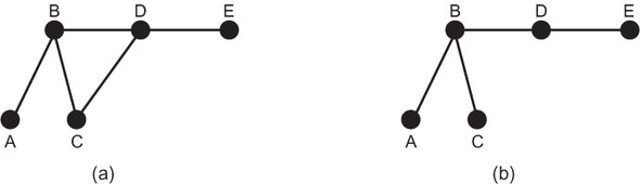
A connected graph is a graph that has some way of getting from any vertex to any other vertex. (All of the graphs we are looking at in this chapter are connected.) A spanning tree is a tree that connects every vertex in a graph. A minimum spanning tree is a tree that connects every vertex in a weighted graph with the minimum total weight (compared to other spanning trees). For every weighted graph, it is possible to efficiently find its minimum spanning tree.
Whew—that was a lot of terminology! The point is that finding a minimum spanning tree is the same as finding a way to connect every vertex in a weighted graph with the minimum weight. This is an important and practical problem for anyone designing a network (transportation network, computer network, and so on): how can every node in the network be connected for the minimum cost? That cost may be in terms of wire, track, road, or anything else. For instance, for a telephone network, another way of posing the problem is “What is the minimum length of cable one needs to connect every phone?”
Revisiting priority queues
Priority queues were covered in chapter 2. We will need a priority queue for Jarník’s algorithm. You can import the PriorityQueue class from chapter 2’s package (see the note immediately previous to listing 4.5 for details), or you can copy the class into a new file to go with this chapter’s package. For completeness, we will recreate Priority-Queue from chapter 2 here, with specific import statements that assume that it will be put in its own stand-alone file.
Listing 4.9. priority_queue.py
from typing import TypeVar, Generic, List
from heapq import heappush, heappop

T = TypeVar('T')

class PriorityQueue(Generic[T]):
    def __init__(self) -> None:
        self._container: List[T] = []

    @property
    def empty(self) -> bool:
        return not self._container  # not is true for empty container

    def push(self, item: T) -> None:
        heappush(self._container, item)  # in by priority

    def pop(self) -> T:
        return heappop(self._container)  # out by priority

    def __repr__(self) -> str:
        return repr(self._container)
Calculating the total weight of a weighted path
Before we develop a method for finding a minimum spanning tree, we will develop a function we can use to test the total weight of a solution. The solution to the minimum spanning tree problem will consist of a list of weighted edges that compose the tree. First, we will define a WeightedPath as a list of WeightedEdge. Then we will define a total_weight() function that takes a list of WeightedPath and finds the total weight that results from adding all of its edges’ weights together.
Listing 4.10. mst.py
from typing import TypeVar, List, Optional
from weighted_graph import WeightedGraph
from weighted_edge import WeightedEdge
from priority_queue import PriorityQueue

V = TypeVar('V') # type of the vertices in the graph
WeightedPath = List[WeightedEdge] # type alias for paths

def total_weight(wp: WeightedPath) -> float:
    return sum([e.weight for e in wp])
Jarník’s algorithm
Jarník’s algorithm for finding a minimum spanning tree works by dividing a graph into two parts: the vertices in the still-being-assembled minimum spanning tree and the vertices not yet in the minimum spanning tree. It takes the following steps:
- Pick an arbitrary vertex to include in the minimum spanning tree.
- Find the lowest-weight edge connecting the minimum spanning tree to the vertices not yet in the minimum spanning tree.
- Add the vertex at the end of that minimum edge to the minimum spanning tree.
- Repeat steps 2 and 3 until every vertex in the graph is in the minimum spanning tree.
Note
Jarník’s algorithm is commonly referred to as Prim’s algorithm. Two Czech mathematicians, Otakar Borůvka and Vojtěch Jarník, interested in minimizing the cost of laying electric lines in the late 1920s, came up with algorithms to solve the problem of finding a minimum spanning tree. Their algorithms were “rediscovered” decades later by others.[3]
Helena Durnová, “Otakar Borůvka (1899-1995) and the Minimum Spanning Tree” (Institute of Mathematics of the Czech Academy of Sciences, 2006), http://mng.bz/O2vj.
To run Jarník’s algorithm efficiently, a priority queue is used. Every time a new vertex is added to the minimum spanning tree, all of its outgoing edges that link to vertices outside the tree are added to the priority queue. The lowest-weight edge is always popped off the priority queue, and the algorithm keeps executing until the priority queue is empty. This ensures that the lowest-weight edges are always added to the tree first. Edges that connect to vertices already in the tree are ignored when they are popped.
The following code for mst() is the full implementation of Jarník’s algorithm,[4] along with a utility function for printing a WeightedPath.
Inspired by a solution by Robert Sedgewick and Kevin Wayne, Algorithms, 4th Edition (Addison-Wesley Professional, 2011), p. 619.
Warning
Jarník’s algorithm will not necessarily work correctly in a graph with directed edges. It also will not work in a graph that is not connected.
Listing 4.11. mst.py continued
def mst(wg: WeightedGraph[V], start: int = 0) -> Optional[WeightedPath]:
    if start > (wg.vertex_count - 1) or start < 0:
        return None
    result: WeightedPath = [] # holds the final MST
    pq: PriorityQueue[WeightedEdge] = PriorityQueue()
    visited: [bool] = [False] * wg.vertex_count # where we've been

    def visit(index: int):
        visited[index] = True # mark as visited
        for edge in wg.edges_for_index(index):
            # add all edges coming from here to pq
            if not visited[edge.v]:
                pq.push(edge)

    visit(start) # the first vertex is where everything begins

    while not pq.empty: # keep going while there are edges to process
        edge = pq.pop()
        if visited[edge.v]:
            continue # don't ever revisit
        # this is the current smallest, so add it to solution
        result.append(edge)
        visit(edge.v) # visit where this connects

    return result

def print_weighted_path(wg: WeightedGraph, wp: WeightedPath) -> None:
    for edge in wp:
        print(f"{wg.vertex_
     at(edge.u)} {edge.weight}> {wg.vertex_at(edge.v)}")
    print(f"Total Weight: {total_weight(wp)}")
Let’s walk through mst(), line by line.
def mst(wg: WeightedGraph[V], start: int = 0) -> Optional[WeightedPath]:
   if start > (wg.vertex_count - 1) or start < 0:
        return None
The algorithm returns an optional WeightedPath representing the minimum spanning tree. It does not matter where the algorithm starts (assuming the graph is connected and undirected), so the default is set to vertex index 0. If it so happens that the start is invalid, mst() returns None.
result: WeightedPath = [] # holds the final MST
pq: PriorityQueue[WeightedEdge] = PriorityQueue()
visited: [bool] = [False] * wg.vertex_count # where we've been
result will ultimately hold the weighted path containing the minimum spanning tree. This is where we will add WeightedEdges, as the lowest-weight edge is popped off and takes us to a new part of the graph. Jarník’s algorithm is considered a greedy algorithm because it always selects the lowest-weight edge. pq is where newly discovered edges are stored and the next-lowest-weight edge is popped. visited keeps track of vertex indices that we have already been to. This could also have been accomplished with a Set, similar to explored in bfs().
def visit(index: int):
    visited[index] = True # mark as visited
    for edge in wg.edges_for_index(index):
        # add all edges coming from here
        if not visited[edge.v]:
            pq.push(edge)
visit() is an inner convenience function that marks a vertex as visited and adds all of its edges that connect to vertices not yet visited to pq. Note how easy the adjacency-list model makes finding edges belonging to a particular vertex.
visit(start) # the first vertex is where everything begins
It does not matter which vertex is visited first unless the graph is not connected. If the graph is not connected, but is instead made up of disconnected components, mst() will return a tree that spans the particular component that the starting vertex belongs to.
while not pq.empty: # keep going while there are edges to process
    edge = pq.pop()
    if visited[edge.v]:
        continue # don't ever revisit
    # this is the current smallest, so add it
    result.append(edge)
    visit(edge.v) # visit where this connects
return result
While there are still edges on the priority queue, we pop them off and check if they lead to vertices not yet in the tree. Because the priority queue is ascending, it pops the lowest-weight edges first. This ensures that the result is indeed of minimum total weight. Any edge popped that does not lead to an unexplored vertex is ignored. Otherwise, because the edge is the lowest seen so far, it is added to the result set, and the new vertex it leads to is explored. When there are no edges left to explore, the result is returned.
Let’s finally return to the problem of connecting all 15 of the largest MSAs in the United States by Hyperloop, using a minimum amount of track. The route that accomplishes this is simply the minimum spanning tree of city_graph2. Let’s try running mst() on city_graph2.
Listing 4.12. mst.py continued
if __name__ == "__main__":
    city_graph2: WeightedGraph[str] = WeightedGraph(["Seattle", "San
     Francisco", "Los Angeles", "Riverside", "Phoenix", "Chicago", "Boston",
     "New York", "Atlanta", "Miami", "Dallas", "Houston", "Detroit",
     "Philadelphia", "Washington"])

    city_graph2.add_edge_by_vertices("Seattle", "Chicago", 1737)
    city_graph2.add_edge_by_vertices("Seattle", "San Francisco", 678)
    city_graph2.add_edge_by_vertices("San Francisco", "Riverside", 386)
    city_graph2.add_edge_by_vertices("San Francisco", "Los Angeles", 348)
    city_graph2.add_edge_by_vertices("Los Angeles", "Riverside", 50)
    city_graph2.add_edge_by_vertices("Los Angeles", "Phoenix", 357)
    city_graph2.add_edge_by_vertices("Riverside", "Phoenix", 307)
    city_graph2.add_edge_by_vertices("Riverside", "Chicago", 1704)
    city_graph2.add_edge_by_vertices("Phoenix", "Dallas", 887)
    city_graph2.add_edge_by_vertices("Phoenix", "Houston", 1015)
    city_graph2.add_edge_by_vertices("Dallas", "Chicago", 805)
    city_graph2.add_edge_by_vertices("Dallas", "Atlanta", 721)
    city_graph2.add_edge_by_vertices("Dallas", "Houston", 225)
    city_graph2.add_edge_by_vertices("Houston", "Atlanta", 702)
    city_graph2.add_edge_by_vertices("Houston", "Miami", 968)
    city_graph2.add_edge_by_vertices("Atlanta", "Chicago", 588)
    city_graph2.add_edge_by_vertices("Atlanta", "Washington", 543)
    city_graph2.add_edge_by_vertices("Atlanta", "Miami", 604)
    city_graph2.add_edge_by_vertices("Miami", "Washington", 923)
    city_graph2.add_edge_by_vertices("Chicago", "Detroit", 238)
    city_graph2.add_edge_by_vertices("Detroit", "Boston", 613)
    city_graph2.add_edge_by_vertices("Detroit", "Washington", 396)
    city_graph2.add_edge_by_vertices("Detroit", "New York", 482)
    city_graph2.add_edge_by_vertices("Boston", "New York", 190)
    city_graph2.add_edge_by_vertices("New York", "Philadelphia", 81)
    city_graph2.add_edge_by_vertices("Philadelphia", "Washington", 123)

    result: Optional[WeightedPath] = mst(city_graph2)
    if result is None:
        print("No solution found!")
    else:
        print_weighted_path(city_graph2, result)
Thanks to the pretty-printing printWeightedPath() method, the minimum spanning tree is easy to read.
Seattle 678> San Francisco
San Francisco 348> Los Angeles
Los Angeles 50> Riverside
Riverside 307> Phoenix
Phoenix 887> Dallas
Dallas 225> Houston
Houston 702> Atlanta
Atlanta 543> Washington
Washington 123> Philadelphia
Philadelphia 81> New York
New York 190> Boston
Washington 396> Detroit
Detroit 238> Chicago
Atlanta 604> Miami
Total Weight: 5372
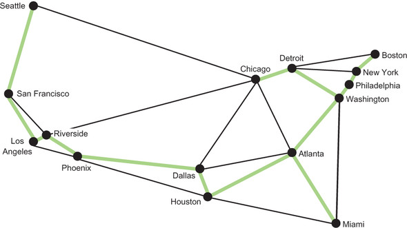
In other words, this is the cumulatively shortest collection of edges that connects all of the MSAs in the weighted graph. The minimum length of track needed to connect all of them is 5,372 miles. Figure 4.7 illustrates the minimum spanning tree.
Figure 4.7. The highlighted edges represent a minimum spanning tree that connects all 15 MSAs.
4.5. Finding shortest paths in a weighted graph
As the Hyperloop network gets built, it is unlikely the builders will have the ambition to connect the whole country at once. Instead, it is likely the builders will want to minimize the cost to lay track between key cities. The cost to extend the network to particular cities will obviously depend on where the builders start.
Finding the cost to any city from some starting city is a version of the “single-source shortest path” problem. That problem asks, “What is the shortest path (in terms of total edge weight) from some vertex to every other vertex in a weighted graph?”
4.5.1. Dijkstra’s algorithm
Dijkstra’s algorithm solves the single-source shortest path problem. It is provided a starting vertex, and it returns the lowest-weight path to any other vertex on a weighted graph. It also returns the minimum total weight to every other vertex from the starting vertex. Dijkstra’s algorithm starts at the single-source vertex and then continually explores the closest vertices to the starting vertex. For this reason, like Jarník’s algorithm, Dijkstra’s algorithm is greedy. When Dijkstra’s algorithm encounters a new vertex, it keeps track of how far it is from the starting vertex and updates this value if it ever finds a shorter path. It also keeps track of which edge got it to each vertex, like a breadth-first search.
Here are all of the algorithm’s steps:
- Add the starting vertex to a priority queue.
- Pop the closest vertex from the priority queue (at the beginning, this is just the starting vertex); we’ll call it the current vertex.
- Look at all of the neighbors connected to the current vertex. If they have not previously been recorded, or if the edge offers a new shortest path to them, then for each of them record its distance from the start, record the edge that produced this distance, and add the new vertex to the priority queue.
- Repeat steps 2 and 3 until the priority queue is empty.
- Return the shortest distance to every vertex from the starting vertex and the path to get to each of them.
The code for Dijkstra’s algorithm includes DijkstraNode, a simple data structure for keeping track of costs associated with each vertex explored so far and for comparing them. This is similar to the Node class in chapter 2. It also includes utility functions for converting the returned array of distances to something easier to use for looking up by vertex and for calculating a shortest path to a particular destination vertex from the path dictionary returned by dijkstra().
Without further ado, here is the code for Dijkstra’s algorithm. We will go over it line by line after.
Listing 4.13. dijkstra.py
from __future__ import annotations
from typing import TypeVar, List, Optional, Tuple, Dict
from dataclasses import dataclass
from mst import WeightedPath, print_weighted_path
from weighted_graph import WeightedGraph
from weighted_edge import WeightedEdge
from priority_queue import PriorityQueue

V = TypeVar('V') # type of the vertices in the graph


@dataclass
class DijkstraNode:
    vertex: int
    distance: float

    def __lt__(self, other: DijkstraNode) -> bool:
        return self.distance < other.distance

    def __eq__(self, other: DijkstraNode) -> bool:
        return self.distance == other.distance

def dijkstra(wg: WeightedGraph[V], root: V) -> Tuple[List[Optional[float]],
     Dict[int, WeightedEdge]]:
    first: int = wg.index_of(root) # find starting index
    # distances are unknown at first
    distances: List[Optional[float]] = [None] * wg.vertex_count
    distances[first] = 0 # the root is 0 away from the root
    path_dict: Dict[int, WeightedEdge] = {} # how we got to each vertex
    pq: PriorityQueue[DijkstraNode] = PriorityQueue()
    pq.push(DijkstraNode(first, 0))

    while not pq.empty:
        u: int = pq.pop().vertex # explore the next closest vertex
        dist_u: float = distances[u] # should already have seen it
        # look at every edge/vertex from the vertex in question
        for we in wg.edges_for_index(u):
            # the old distance to this vertex
            dist_v: float = distances[we.v]
            # no old distance or found shorter path
            if dist_v is None or dist_v > we.weight + dist_u:
                # update distance to this vertex
                distances[we.v] = we.weight + dist_u
                # update the edge on the shortest path to this vertex
                path_dict[we.v] = we
                # explore it soon
                pq.push(DijkstraNode(we.v, we.weight + dist_u))

    return distances, path_dict

# Helper function to get easier access to dijkstra results
def distance_array_to_vertex_dict(wg: WeightedGraph[V], distances:
     List[Optional[float]]) -> Dict[V, Optional[float]]:
    distance_dict: Dict[V, Optional[float]] = {}
    for i in range(len(distances)):
        distance_dict[wg.vertex_at(i)] = distances[i]
    return distance_dict

# Takes a dictionary of edges to reach each node and returns a list of
# edges that goes from `start` to `end`
def path_dict_to_path(start: int, end: int, path_dict: Dict[int,
     WeightedEdge]) -> WeightedPath:
    if len(path_dict) == 0:
        return []
    edge_path: WeightedPath = []
    e: WeightedEdge = path_dict[end]
    edge_path.append(e)
    while e.u != start:
        e = path_dict[e.u]
        edge_path.append(e)
    return list(reversed(edge_path))
The first few lines of dijkstra() use data structures you have become familiar with, except for distances, which is a placeholder for the distances to every vertex in the graph from the root. Initially all of these distances are None, because we do not yet know how far each of them is; that is what we are using Dijkstra’s algorithm to figure out!
def dijkstra(wg: WeightedGraph[V], root: V) -> Tuple[List[Optional[float]],
     Dict[int, WeightedEdge]]:
    first: int = wg.index_of(root) # find starting index
    # distances are unknown at first
    distances: List[Optional[float]] = [None] * wg.vertex_count
    distances[first] = 0 # the root is 0 away from the root
    path_dict: Dict[int, WeightedEdge] = {} # how we got to each vertex
    pq: PriorityQueue[DijkstraNode] = PriorityQueue()
    pq.push(DijkstraNode(first, 0))
The first node pushed onto the priority queue contains the root vertex.
while not pq.empty:
    u: int = pq.pop().vertex # explore the next closest vertex
    dist_u: float = distances[u] # should already have seen it
We keep running Dijkstra’s algorithm until the priority queue is empty. u is the current vertex we are searching from, and dist_u is the stored distance for getting to u along known routes. Every vertex explored at this stage has already been found, so it must have a known distance.
# look at every edge/vertex from here
for we in wg.edges_for_index(u):
    # the old distance to this
    dist_v: float = distances[we.v]
Next, every edge connected to u is explored. dist_v is the distance to any known vertex attached by an edge from u.
# no old distance or found shorter path
if dist_v is None or dist_v > we.weight + dist_u:
    # update distance to this vertex
    distances[we.v] = we.weight + dist_u
    # update the edge on the shortest path
    path_dict[we.v] = we
    # explore it soon
    pq.push(DijkstraNode(we.v, we.weight + dist_u))
If we have found a vertex that has not yet been explored (dist_v is None), or we have found a new, shorter path to it, we record that new shortest distance to v and the edge that got us there. Finally, we push any vertices that have new paths to them to the priority queue.
return distances, path_dict
dijkstra() returns both the distances to every vertex in the weighted graph from the root vertex, and the path_dict that can unlock the shortest paths to them.
It is safe to run Dijkstra’s algorithm now. We will start by finding the distance from Los Angeles to every other MSA in the graph. Then we will find the shortest path between Los Angeles and Boston. Finally, we will use print_weighted_path() to pretty-print the result.
Listing 4.14. dijkstra.py continued
if __name__ == "__main__":
    city_graph2: WeightedGraph[str] = WeightedGraph(["Seattle", "San
     Francisco", "Los Angeles", "Riverside", "Phoenix", "Chicago", "Boston",
     "New York", "Atlanta", "Miami", "Dallas", "Houston", "Detroit",
     "Philadelphia", "Washington"])

    city_graph2.add_edge_by_vertices("Seattle", "Chicago", 1737)
    city_graph2.add_edge_by_vertices("Seattle", "San Francisco", 678)
    city_graph2.add_edge_by_vertices("San Francisco", "Riverside", 386)
    city_graph2.add_edge_by_vertices("San Francisco", "Los Angeles", 348)
    city_graph2.add_edge_by_vertices("Los Angeles", "Riverside", 50)
    city_graph2.add_edge_by_vertices("Los Angeles", "Phoenix", 357)
    city_graph2.add_edge_by_vertices("Riverside", "Phoenix", 307)
    city_graph2.add_edge_by_vertices("Riverside", "Chicago", 1704)
    city_graph2.add_edge_by_vertices("Phoenix", "Dallas", 887)
    city_graph2.add_edge_by_vertices("Phoenix", "Houston", 1015)
    city_graph2.add_edge_by_vertices("Dallas", "Chicago", 805)
    city_graph2.add_edge_by_vertices("Dallas", "Atlanta", 721)
    city_graph2.add_edge_by_vertices("Dallas", "Houston", 225)
    city_graph2.add_edge_by_vertices("Houston", "Atlanta", 702)
    city_graph2.add_edge_by_vertices("Houston", "Miami", 968)
    city_graph2.add_edge_by_vertices("Atlanta", "Chicago", 588)
    city_graph2.add_edge_by_vertices("Atlanta", "Washington", 543)
    city_graph2.add_edge_by_vertices("Atlanta", "Miami", 604)
    city_graph2.add_edge_by_vertices("Miami", "Washington", 923)
    city_graph2.add_edge_by_vertices("Chicago", "Detroit", 238)
    city_graph2.add_edge_by_vertices("Detroit", "Boston", 613)
    city_graph2.add_edge_by_vertices("Detroit", "Washington", 396)
    city_graph2.add_edge_by_vertices("Detroit", "New York", 482)
    city_graph2.add_edge_by_vertices("Boston", "New York", 190)
    city_graph2.add_edge_by_vertices("New York", "Philadelphia", 81)
    city_graph2.add_edge_by_vertices("Philadelphia", "Washington", 123)

    distances, path_dict = dijkstra(city_graph2, "Los Angeles")
    name_distance: Dict[str, Optional[int]] = distance_array_to_vertex_
     dict(city_graph2, distances)
    print("Distances from Los Angeles:")
    for key, value in name_distance.items():
        print(f"{key} : {value}")
    print("") # blank line

    print("Shortest path from Los Angeles to Boston:")
    path: WeightedPath = path_dict_to_path(city_graph2.index_of("Los
     Angeles"), city_graph2.index_of("Boston"), path_dict)
    print_weighted_path(city_graph2, path)
Your output should look something like this:
Distances from Los Angeles:
Seattle : 1026
San Francisco : 348
Los Angeles : 0
Riverside : 50
Phoenix : 357
Chicago : 1754
Boston : 2605
New York : 2474
Atlanta : 1965
Miami : 2340
Dallas : 1244
Houston : 1372
Detroit : 1992
Philadelphia : 2511
Washington : 2388

Shortest path from Los Angeles to Boston:
Los Angeles 50> Riverside
Riverside 1704> Chicago
Chicago 238> Detroit
Detroit 613> Boston
Total Weight: 2605
You may have noticed that Dijkstra’s algorithm has some resemblance to Jarník’s algorithm. They are both greedy, and it is possible to implement them using quite similar code if one is sufficiently motivated. Another algorithm that Dijkstra’s algorithm resembles is A* from chapter 2. A* can be thought of as a modification of Dijkstra’s algorithm. Add a heuristic and restrict Dijkstra’s algorithm to finding a single destination, and the two algorithms are the same.
Note
Dijkstra’s algorithm is designed for graphs with positive weights. Graphs with negatively weighted edges can pose a challenge for Dijkstra’s algorithm and will require modification or an alternative algorithm.
4.6. Real-world applications
A huge amount of our world can be represented using graphs. You have seen in this chapter how effective they are for working with transportation networks, but many other kinds of networks have the same essential optimization problems: telephone networks, computer networks, utility networks (electricity, plumbing, and so on). As a result, graph algorithms are essential for efficiency in the telecommunications, shipping, transportation, and utility industries.
Retailers must handle complex distribution problems. Stores and warehouses can be thought of as vertices and the distances between them as edges. The algorithms are the same. The internet itself is a giant graph, with each connected device a vertex and each wired or wireless connection being an edge. Whether a business is saving fuel or wire, minimum spanning tree and shortest path problem-solving are useful for more than just games. Some of the world’s most famous brands became successful by optimizing graph problems: think of Walmart building out an efficient distribution network, Google indexing the web (a giant graph), and FedEx finding the right set of hubs to connect the world’s addresses.
Some obvious applications of graph algorithms are social networks and map applications. In a social network, people are vertices, and connections (friendships on Facebook, for instance) are edges. In fact, one of Facebook’s most prominent developer tools is known as the Graph API (https://developers.facebook.com/docs/graph-api). In map applications like Apple Maps and Google Maps, graph algorithms are used to provide directions and calculate trip times.
Several popular video games also make explicit use of graph algorithms. Mini-Metro and Ticket to Ride are two examples of games that closely mimic the problems solved in this chapter.
4.7. Exercises
- Add support to the graph framework for removing edges and vertices.
- Add support to the graph framework for directed graphs (digraphs).
- Use this chapter’s graph framework to prove or disprove the classic Bridges of Königsberg problem, as described on Wikipedia: https://en.wikipedia.org/wiki/Seven_Bridges_of_Königsberg.