Chapter 2. Search problems
“Search” is such a broad term that this entire book could be called Classic Search Problems in Python. This chapter is about core search algorithms that every programmer should know. It does not claim to be comprehensive, despite the declaratory title.
2.1. DNA search
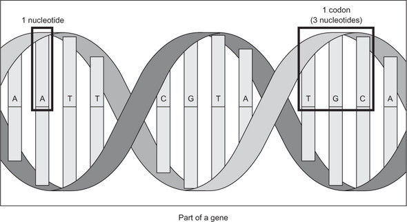
Genes are commonly represented in computer software as a sequence of the characters A, C, G, and T. Each letter represents a nucleotide, and the combination of three nucleotides is called a codon. This is illustrated in figure 2.1. A codon codes for a specific amino acid that together with other amino acids can form a protein. A classic task in bioinformatics software is to find a particular codon within a gene.
2.1.1. Storing DNA
We can represent a nucleotide as a simple IntEnum with four cases.
Listing 2.1. dna_search.py
from enum import IntEnum
from typing import Tuple, List

Nucleotide: IntEnum = IntEnum('Nucleotide', ('A', 'C', 'G', 'T'))
Figure 2.1. A nucleotide is represented by one of the letters A, C, G, and T. A codon is composed of three nucleotides, and a gene is composed of multiple codons.
Nucleotide is of type IntEnum instead of just Enum, because IntEnum gives us comparison operators (<, >=, and so on) “for free.” Having these operators in a data type is required in order for the search algorithms we are going to implement to be able to operate on it. Tuple and List are imported from the typing package to assist with type hints.
Codons can be defined as a tuple of three Nucleotides. A gene may be defined as a list of Codons.
Listing 2.2. dna_search.py continued
Codon = Tuple[Nucleotide, Nucleotide, Nucleotide]  # type alias for codons
Gene = List[Codon]  # type alias for genes
Note
Although we will later need to compare one Codon to another, we do not need to define a custom class with the < operator explicitly implemented for Codon. This is because Python has built-in support for comparisons between tuples that are composed of types that are also comparable.
Typically, genes on the internet will be in a file format that contains a giant string representing all of the nucleotides in the gene’s sequence. We will define such a string for an imaginary gene and call it gene_str.
Listing 2.3. dna_search.py continued
gene_str: str = "ACGTGGCTCTCTAACGTACGTACGTACGGGGTTTATATATACCCTAGGACTCCCTTT"
We will also need a utility function to convert a str into a Gene.
Listing 2.4. dna_search.py continued
def string_to_gene(s: str) -> Gene:
    gene: Gene = []
    for i in range(0, len(s), 3):
        if (i + 2) >= len(s):  # don't run off end!
            return gene
        #  initialize codon out of three nucleotides
        codon: Codon = (Nucleotide[s[i]], Nucleotide[s[i + 1]], Nucleotide[s[i + 2]])
        gene.append(codon)  # add codon to gene
    return gene
string_to_gene() continually goes through the provided str and converts its next three characters into Codons that it adds to the end of a new Gene. If it finds that there is no Nucleotide two places into the future of the current place in s that it is examining (see the if statement within the loop), then it knows it has reached the end of an incomplete gene, and it skips over those last one or two nucleotides.
string_to_gene() can be used to convert the str gene_str into a Gene.
Listing 2.5. dna_search.py continued
my_gene: Gene = string_to_gene(gene_str)
2.1.2. Linear search
One basic operation we may want to perform on a gene is to search it for a particular codon. The goal is to simply find out whether the codon exists within the gene or not.
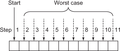
A linear search goes through every element in a search space, in the order of the original data structure, until what is sought is found or the end of the data structure is reached. In effect, a linear search is the most simple, natural, and obvious way to search for something. In the worst case, a linear search will require going through every element in a data structure, so it is of O(n) complexity, where n is the number of elements in the structure. This is illustrated in figure 2.2.
Figure 2.2. In the worst case of a linear search, you’ll sequentially look through every element of the array.
It is trivial to define a function that performs a linear search. It simply must go through every element in a data structure and check for its equivalence to the item being sought. The following code defines such a function for a Gene and a Codon and then tries it out for my_gene and Codons called acg and gat.
Listing 2.6. dna_search.py continued
def linear_contains(gene: Gene, key_codon: Codon) -> bool:
    for codon in gene:
        if codon == key_codon:
            return True
    return False
acg: Codon = (Nucleotide.A, Nucleotide.C, Nucleotide.G)
gat: Codon = (Nucleotide.G, Nucleotide.A, Nucleotide.T)
print(linear_contains(my_gene, acg))  # True
print(linear_contains(my_gene, gat))  # False
Note
This function is for illustrative purposes only. The Python built-in sequence types (list, tuple, range) all implement the __contains__() method, which allows us to do a search for a specific item in them by simply using the in operator. In fact, the in operator can be used with any type that implements __contains__(). For instance, we could search my_gene for acg and print out the result by writing print(acg in my_gene).
2.1.3. Binary search
There is a faster way to search than looking at every element, but it requires us to know something about the order of the data structure ahead of time. If we know that the structure is sorted, and we can instantly access any item within it by its index, we can perform a binary search. Based on this criteria, a sorted Python list is a perfect candidate for a binary search.
A binary search works by looking at the middle element in a sorted range of elements, comparing it to the element sought, reducing the range by half based on that comparison, and starting the process over again. Let’s look at a concrete example.
Suppose we have a list of alphabetically sorted words like ["cat", "dog", "kangaroo", "llama", "rabbit", "rat", "zebra"] and we are searching for the word “rat”:
- We could determine that the middle element in this seven-word list is “llama.”
- We could determine that “rat” comes after “llama” alphabetically, so it must be in the (approximately) half of the list that comes after “llama.” (If we had found “rat” in this step, we could have returned its location; if we had found that our word came before the middle word we were checking, we could be assured that it was in the half of the list before “llama.”)
- We could rerun steps 1 and 2 for the half of the list that we know “rat” is still possibly in. In effect, this half becomes our new base list. These steps continually run until “rat” is found or the range we are looking in no longer contains any elements to search, meaning that “rat” does not exist within the word list.
Figure 2.3 illustrates a binary search. Notice that it does not involve searching every element, unlike a linear search.
Figure 2.3. In the worst case of a binary search, you’ll look through just lg(n) elements of the list.
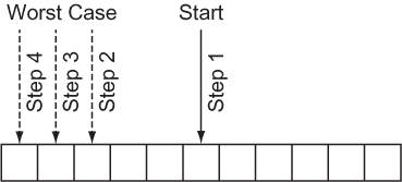
A binary search continually reduces the search space by half, so it has a worst-case runtime of O(lg n). There is a sort-of catch, though. Unlike a linear search, a binary search requires a sorted data structure to search through, and sorting takes time. In fact, sorting takes O(n lg n) time for the best sorting algorithms. If we are only going to run our search once, and our original data structure is unsorted, it probably makes sense to just do a linear search. But if the search is going to be performed many times, the time cost of doing the sort is worth it, to reap the benefit of the greatly reduced time cost of each individual search.
Writing a binary search function for a gene and a codon is not unlike writing one for any other type of data, because the Codon type can be compared to others of its type, and the Gene type is just a list.
Listing 2.7. dna_search.py continued
def binary_contains(gene: Gene, key_codon: Codon) -> bool:
    low: int = 0
    high: int = len(gene) - 1
    while low <= high:  # while there is still a search space
        mid: int = (low + high) // 2
        if gene[mid] < key_codon:
            low = mid + 1
        elif gene[mid] > key_codon:
            high = mid - 1
        else:
            return True
    return False
Let’s walk through this function line by line.
low: int = 0
high: int = len(gene) - 1
We start by looking at a range that encompasses the entire list (gene).
while low <= high:
We keep searching as long as there is a still a range to search within. When low is greater than high, it means that there are no longer any slots to look at within the list.
mid: int = (low + high) // 2
We calculate the middle, mid, by using integer division and the simple mean formula you learned in grade school.
if gene[mid] < key_codon:
    low = mid + 1
If the element we are looking for is after the middle element of the range we are looking at, we modify the range that we will look at during the next iteration of the loop by moving low to be one past the current middle element. This is where we halve the range for the next iteration.
elif gene[mid] > key_codon:
    high = mid - 1
Similarly, we halve in the other direction when the element we are looking for is less than the middle element.
else:
    return True
If the element in question is not less than or greater than the middle element, that means we found it! And, of course, if the loop ran out of iterations, we return False (not reproduced here), indicating that it was never found.
We can try running our function with the same gene and codon, but we must remember to sort first.
Listing 2.8. dna_search.py continued
my_sorted_gene: Gene = sorted(my_gene)
print(binary_contains(my_sorted_gene, acg))  # True
print(binary_contains(my_sorted_gene, gat))  # False
TIP
You can build a performant binary search using the Python standard library’s bisect module: https://docs.python.org/3/library/bisect.html.
2.1.4. A generic example
The functions linear_contains() and binary_contains() can be generalized to work with almost any Python sequence. The following generalized versions are nearly identical to the versions you saw before, with only some names and type hints changed.
Note
There are many imported types in the following code listing. We will be reusing the file generic_search.py for many further generic search algorithms in this chapter, and this gets the imports out of the way.
Note
Before proceeding with the book, you will need to install the typing_extensions module via either pip install typing_extensions or pip3 install typing_extensions, depending on how your Python interpreter is configured. You will need this module to access the Protocol type, which will be in the standard library in a future version of Python (as specified by PEP 544). Therefore, in a future version of Python, importing the typing_extensions module should be unnecessary, and you will be able to use from typing import Protocol instead of from typing_extensions import Protocol.
Listing 2.9. generic_search.py
from __future__ import annotations
from typing import TypeVar, Iterable, Sequence, Generic, List, Callable, Set,
     Deque, Dict, Any, Optional
from typing_extensions import Protocol
from heapq import heappush, heappop

T = TypeVar('T')
def linear_contains(iterable: Iterable[T], key: T) -> bool:
    for item in iterable:
        if item == key:
            return True
    return False

C = TypeVar("C", bound="Comparable")

class Comparable(Protocol):
    def __eq__(self, other: Any) -> bool:
        ...

    def __lt__(self: C, other: C) -> bool:
        ...

    def __gt__(self: C, other: C) -> bool:
        return (not self < other) and self != other

    def __le__(self: C, other: C) -> bool:
        return self < other or self == other

    def __ge__(self: C, other: C) -> bool:
        return not self < other


def binary_contains(sequence: Sequence[C], key: C) -> bool:
    low: int = 0
    high: int = len(sequence) - 1
    while low <= high:  # while there is still a search space
        mid: int = (low + high) // 2
        if sequence[mid] < key:
            low = mid + 1
        elif sequence[mid] > key:
            high = mid - 1
        else:
            return True
    return False

if __name__ == "__main__":
    print(linear_contains([1, 5, 15, 15, 15, 15, 20], 5))  # True
    print(binary_contains(["a", "d", "e", "f", "z"], "f"))  # True
    print(binary_contains(["john", "mark", "ronald", "sarah"], "sheila"))  #
     False
Now you can try doing searches on other types of data. These functions can be reused for almost any Python collection. That is the power of writing code generically. The only unfortunate element of this example is the convoluted hoops that had to be jumped through for Python’s type hints, in the form of the Comparable class. A Comparable type is a type that implements the comparison operators (<, >=, and so on). There should be a more succinct way in future versions of Python to create a type hint for types that implement these common operators.
2.2. Maze solving
Finding a path through a maze is analogous to many common search problems in computer science. Why not literally find a path through a maze, then, to illustrate the breadth-first search, depth-first search, and A* algorithms?
Our maze will be a two-dimensional grid of Cells. A Cell is an enum with str values where " " will represent an empty space and "X" will represent a blocked space. There are also other cases for illustrative purposes when printing a maze.
Listing 2.10. maze.py
from enum import Enum
from typing import List, NamedTuple, Callable, Optional
import random
from math import sqrt
from generic_search import dfs, bfs, node_to_path, astar, Node

class Cell(str, Enum):
    EMPTY = " "
    BLOCKED = "X"
    START = "S"
    GOAL = "G"
    PATH = "*"
Once again, we are getting a large number of imports out of the way. Note that the last import (from generic_search) is of symbols we have not yet defined. It is included here for convenience, but you may want to comment it out until you need it.
We will need a way to refer to an individual location in the maze. This will simply be a NamedTuple with properties representing the row and column of the location in question.
Listing 2.11. maze.py continued
class MazeLocation(NamedTuple):
    row: int
    column: int
2.2.1. Generating a random maze
Our Maze class will internally keep track of a grid (a list of lists) representing its state. It will also have instance variables for the number of rows, number of columns, start location, and goal location. Its grid will be randomly filled with blocked cells.
The maze that is generated should be fairly sparse so that there is almost always a path from a given starting location to a given goal location. (This is for testing our algorithms, after all.) We’ll let the caller of a new maze decide on the exact sparseness, but we will provide a default value of 20% blocked. When a random number beats the threshold of the sparseness parameter in question, we will simply replace an empty space with a wall. If we do this for every possible place in the maze, statistically, the sparseness of the maze as a whole will approximate the sparseness parameter supplied.
Listing 2.12. maze.py continued
class Maze:
    def __init__(self, rows: int = 10, columns: int = 10, sparseness: float =
     0.2, start: MazeLocation = MazeLocation(0, 0), goal: MazeLocation =
     MazeLocation(9, 9)) -> None:
        # initialize basic instance variables
        self._rows: int = rows
        self._columns: int = columns
        self.start: MazeLocation = start
        self.goal: MazeLocation = goal
        # fill the grid with empty cells
        self._grid: List[List[Cell]] = [[Cell.EMPTY for c in range(columns)]
     for r in range(rows)]
        # populate the grid with blocked cells
        self._randomly_fill(rows, columns, sparseness)
        # fill the start and goal locations in
        self._grid[start.row][start.column] = Cell.START
        self._grid[goal.row][goal.column] = Cell.GOAL

    def _randomly_fill(self, rows: int, columns: int, sparseness: float):
        for row in range(rows):
            for column in range(columns):
                if random.uniform(0, 1.0) < sparseness:
                    self._grid[row][column] = Cell.BLOCKED
Now that we have a maze, we also want a way to print it succinctly to the console. We want its characters to be close together so it looks like a real maze.
Listing 2.13. maze.py continued
# return a nicely formatted version of the maze for printing
def __str__(self) -> str:
    output: str = ""
    for row in self._grid:
        output += "".join([c.value for c in row]) + "\n"
    return output
Go ahead and test these maze functions.
maze: Maze = Maze()
print(maze)
2.2.2. Miscellaneous maze minutiae
It will be handy later to have a function that checks whether we have reached our goal during the search. In other words, we want to check whether a particular Maze-Location that the search has reached is the goal. We can add a method to Maze.
Listing 2.14. maze.py continued
def goal_test(self, ml: MazeLocation) -> bool:
    return ml == self.goal
How can we move within our mazes? Let’s say that we can move horizontally and vertically one space at a time from a given space in the maze. Using these criteria, a successors() function can find the possible next locations from a given MazeLocation. However, the successors() function will differ for every Maze because every Maze has a different size and set of walls. Therefore, we will define it as a method on Maze.
Listing 2.15. maze.py continued
def successors(self, ml: MazeLocation) -> List[MazeLocation]:
    locations: List[MazeLocation] = []
    if ml.row + 1 < self._rows and self._grid[ml.row + 1][ml.column] !=
     Cell.BLOCKED:
        locations.append(MazeLocation(ml.row + 1, ml.column))
    if ml.row - 1 >= 0 and self._grid[ml.row - 1][ml.column] != Cell.BLOCKED:
        locations.append(MazeLocation(ml.row - 1, ml.column))
    if ml.column + 1 < self._columns and self._grid[ml.row][ml.column + 1] !=
     Cell.BLOCKED:
        locations.append(MazeLocation(ml.row, ml.column + 1))
    if ml.column - 1 >= 0 and self._grid[ml.row][ml.column - 1] !=
     Cell.BLOCKED:
        locations.append(MazeLocation(ml.row, ml.column - 1))
    return locations
successors() simply checks above, below, to the right, and to the left of a Maze-Location in a Maze to see if it can find empty spaces that can be gone to from that location. It also avoids checking locations beyond the edges of the Maze. It puts every possible MazeLocation that it finds into a list that it ultimately returns to the caller.
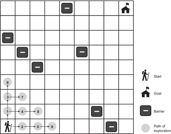
2.2.3. Depth-first search
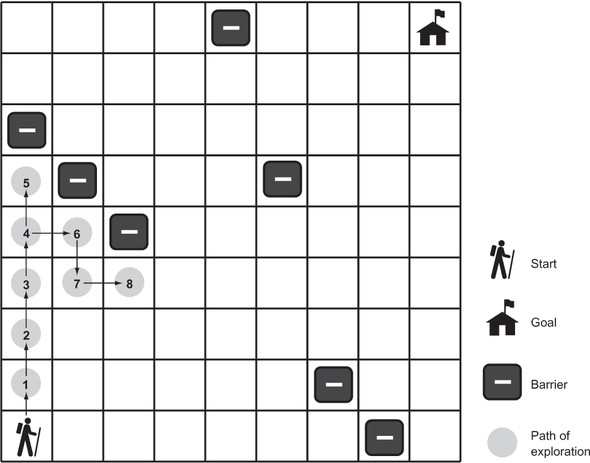
A depth-first search (DFS) is what its name suggests: a search that goes as deeply as it can before backtracking to its last decision point if it reaches a dead end. We’ll implement a generic depth-first search that can solve our maze problem. It will also be reusable for other problems. Figure 2.4 illustrates an in-progress depth-first search of a maze.
Figure 2.4. In depth-first search, the search proceeds along a continuously deeper path until it hits a barrier and must backtrack to the last decision point.
Stacks
The depth-first search algorithm relies on a data structure known as a stack. (If you read about stacks in chapter 1, feel free to skip this section.) A stack is a data structure that operates under the Last-In-First-Out (LIFO) principle. Imagine a stack of papers. The last paper placed on top of the stack is the first paper pulled off the stack. It is common for a stack to be implemented on top of a more primitive data structure like a list. We will implement our stack on top of Python’s list type.
Stacks generally have at least two operations:
- push()—Places an item on top of the stack
- pop()—Removes the item from the top of the stack and returns it
We will implement both of these, as well as an empty property to check if the stack has any more items in it. We will add the code for the stack to the generic_search.py file that we were working with earlier in the chapter. We already have completed all of the necessary imports.
Listing 2.16. generic_search.py continued
class Stack(Generic[T]):
    def __init__(self) -> None:
        self._container: List[T] = []

    @property
    def empty(self) -> bool:
        return not self._container  # not is true for empty container

    def push(self, item: T) -> None:
        self._container.append(item)

    def pop(self) -> T:
        return self._container.pop()  # LIFO

    def __repr__(self) -> str:
        return repr(self._container)
Note that implementing a stack using a Python list is as simple as always appending items onto its right end and always removing items from its extreme right end. The pop() method on list will fail if there are no longer any items in the list, so pop() will fail on a Stack if it is empty as well.
The DFS algorithm
We will need one more little tidbit before we can get to implementing DFS. We need a Node class that we will use to keep track of how we got from one state to another state (or from one place to another place) as we search. You can think of a Node as a wrapper around a state. In the case of our maze-solving problem, those states are of type MazeLocation. We’ll call the Node that a state came from its parent. We will also define our Node class as having cost and heuristic properties and with __lt__() implemented, so we can reuse it later in the A* algorithm.
Listing 2.17. generic_search.py continued
class Node(Generic[T]):
    def __init__(self, state: T, parent: Optional[Node], cost: float = 0.0,
     heuristic: float = 0.0) -> None:
        self.state: T = state
        self.parent: Optional[Node] = parent
        self.cost: float = cost
        self.heuristic: float = heuristic

    def __lt__(self, other: Node) -> bool:
        return (self.cost + self.heuristic) < (other.cost + other.heuristic)
TIP
The Optional type indicates that a value of a parameterized type may be referenced by the variable, or the variable may reference None.
TIP
At the top of the file, the from __future__ import annotations allows Node to reference itself in the type hints of its methods. Without it, we would need to put the type hint in quotes as a string (for example, 'Node'). In future versions of Python, importing annotations will be unnecessary. See PEP 563, “Postponed Evaluation of Annotations,” for more information: http://mng.bz/pgzR.
An in-progress depth-first search needs to keep track of two data structures: the stack of states (or “places”) that we are considering searching, which we will call the frontier; and the set of states that we have already searched, which we will call explored. As long as there are more states to visit in the frontier, DFS will keep checking whether they are the goal (if a state is the goal, DFS will stop and return it) and adding their successors to the frontier. It will also mark each state that has already been searched as explored, so that the search does not get caught in a circle, reaching states that have prior visited states as successors. If the frontier is empty, it means there is nowhere left to search.
Listing 2.18. generic_search.py continued
def dfs(initial: T, goal_test: Callable[[T], bool], successors: Callable[[T],
     List[T]]) -> Optional[Node[T]]:
    # frontier is where we've yet to go
    frontier: Stack[Node[T]] = Stack()
    frontier.push(Node(initial, None))
    # explored is where we've been
    explored: Set[T] = {initial}

    # keep going while there is more to explore
    while not frontier.empty:
        current_node: Node[T] = frontier.pop()
        current_state: T = current_node.state
        # if we found the goal, we're done
        if goal_test(current_state):
            return current_node
        # check where we can go next and haven't explored
        for child in successors(current_state):
            if child in explored:  # skip children we already explored
                continue
            explored.add(child)
            frontier.push(Node(child, current_node))
    return None  # went through everything and never found goal
If dfs() is successful, it returns the Node encapsulating the goal state. The path from the start to the goal can be reconstructed by working backward from this Node and its priors using the parent property.
Listing 2.19. generic_search.py continued
def node_to_path(node: Node[T]) -> List[T]:
    path: List[T] = [node.state]
    # work backwards from end to front
    while node.parent is not None:
        node = node.parent
        path.append(node.state)
    path.reverse()
    return path
For display purposes, it will be useful to mark up the maze with the successful path, the start state, and the goal state. It will also be useful to be able to remove a path so that we can try different search algorithms on the same maze. The following two methods should be added to the Maze class in maze.py.
Listing 2.20. maze.py continued
def mark(self, path: List[MazeLocation]):
    for maze_location in path:
        self._grid[maze_location.row][maze_location.column] = Cell.PATH
    self._grid[self.start.row][self.start.column] = Cell.START
    self._grid[self.goal.row][self.goal.column] = Cell.GOAL

def clear(self, path: List[MazeLocation]):
    for maze_location in path:
        self._grid[maze_location.row][maze_location.column] = Cell.EMPTY
    self._grid[self.start.row][self.start.column] = Cell.START
    self._grid[self.goal.row][self.goal.column] = Cell.GOAL
It has been a long journey, but we are finally ready to solve the maze.
Listing 2.21. maze.py continued
if __name__ == "__main__":
    # Test DFS
    m: Maze = Maze()
    print(m)
    solution1: Optional[Node[MazeLocation]] = dfs(m.start, m.goal_test,
     m.successors)
    if solution1 is None:
        print("No solution found using depth-first search!")
    else:
        path1: List[MazeLocation] = node_to_path(solution1)
        m.mark(path1)
        print(m)
        m.clear(path1)
A successful solution will look something like this:
S****X X
 X  *****
       X*
 XX******X
  X*
  X**X
 X  *****
        *
     X  *X
        *G
The asterisks represent the path that our depth-first search function found from the start to the goal. Remember, because each maze is randomly generated, not every maze has a solution.
2.2.4. Breadth-first search
You may notice that the solution paths to the mazes found by depth-first traversal seem unnatural. They are usually not the shortest paths. Breadth-first search (BFS) always finds the shortest path by systematically looking one layer of nodes farther away from the start state in each iteration of the search. There are particular problems in which a depth-first search is likely to find a solution more quickly than a breadth-first search, and vice versa. Therefore, choosing between the two is sometimes a trade-off between the possibility of finding a solution quickly and the certainty of finding the shortest path to the goal (if one exists). Figure 2.5 illustrates an in-progress breadth-first search of a maze.
Figure 2.5. In a breadth-first search, the closest elements to the starting location are searched first.
To understand why a depth-first search sometimes returns a result faster than a breadth-first search, imagine looking for a marking on a particular layer of an onion. A searcher using a depth-first strategy may plunge a knife into the center of the onion and haphazardly examine the chunks cut out. If the marked layer happens to be near the chunk cut out, there is a chance that the searcher will find it more quickly than another searcher using a breadth-first strategy, who painstakingly peels the onion one layer at a time.
To get a better picture of why breadth-first search always finds the shortest solution path where one exists, consider trying to find the path with the fewest number of stops between Boston and New York by train. If you keep going in the same direction and backtracking when you hit a dead end (as in depth-first search), you may first find a route all the way to Seattle before it connects back to New York. However, in a breadth-first search, you will first check all of the stations one stop away from Boston. Then you will check all of the stations two stops away from Boston. Then you will check all of the stations three stops away from Boston. This will keep going until you find New York. Therefore, when you do find New York, you will know you have found the route with the fewest stops, because you already checked all of the stations that are fewer stops away from Boston, and none of them was New York.
Queues
To implement BFS, a data structure known as a queue is required. Whereas a stack is LIFO, a queue is FIFO (First-In-First-Out). A queue is like a line to use a restroom. The first person who got in line goes to the restroom first. At a minimum, a queue has the same push() and pop() methods as a stack. In fact, our implementation for Queue (backed by a Python deque) is almost identical to our implementation of Stack, with the only changes being the removal of elements from the left end of the _container instead of the right end and the switch from a list to a deque. (I use the word “left” here to mean the beginning of the backing store.) The elements on the left end are the oldest elements still in the deque (in terms of arrival time), so they are the first elements popped.
Listing 2.22. generic_search.py continued
class Queue(Generic[T]):
    def __init__(self) -> None:
        self._container: Deque[T] = Deque()

    @property
    def empty(self) -> bool:
        return not self._container  # not is true for empty container

    def push(self, item: T) -> None:
        self._container.append(item)

    def pop(self) -> T:
        return self._container.popleft()  # FIFO

    def __repr__(self) -> str:
        return repr(self._container)
TIP
Why did the implementation of Queue use a deque as its backing store, whereas the implementation of Stack used a list as its backing store? It has to do with where we pop. In a stack, we push to the right and pop from the right. In a queue we push to the right as well, but we pop from the left. The Python list data structure has efficient pops from the right but not from the left. A deque can efficiently pop from either side. As a result, there is a built-in method on deque called popleft() but no equivalent method on list. You could certainly find other ways to use a list as the backing store for a queue, but they would be less efficient. Popping from the left on a deque is an O(1) operation, whereas it is an O(n) operation on a list. In the case of the list, after popping from the left, every subsequent element must be moved one to the left, making it inefficient.
The BFS algorithm
Amazingly, the algorithm for a breadth-first search is identical to the algorithm for a depth-first search, with the frontier changed from a stack to a queue. Changing the frontier from a stack to a queue changes the order in which states are searched and ensures that the states closest to the start state are searched first.
Listing 2.23. generic_search.py continued
def bfs(initial: T, goal_test: Callable[[T], bool], successors: Callable[[T],
     List[T]]) -> Optional[Node[T]]:
    # frontier is where we've yet to go
    frontier: Queue[Node[T]] = Queue()
    frontier.push(Node(initial, None))
    # explored is where we've been
    explored: Set[T] = {initial}

    # keep going while there is more to explore
    while not frontier.empty:
        current_node: Node[T] = frontier.pop()
        current_state: T = current_node.state
        # if we found the goal, we're done
        if goal_test(current_state):
            return current_node
        # check where we can go next and haven't explored
        for child in successors(current_state):
            if child in explored:  # skip children we already explored
                continue
            explored.add(child)
            frontier.push(Node(child, current_node))
    return None  # went through everything and never found goal
If you try running bfs(), you will see that it always finds the shortest solution to the maze in question. The following trial is added just after the previous one in the if __name__ == "__main__": section of the file, so results can be compared on the same maze.
Listing 2.24. maze.py continued
# Test BFS
solution2: Optional[Node[MazeLocation]] = bfs(m.start, m.goal_test,
     m.successors)
if solution2 is None:
    print("No solution found using breadth-first search!")
else:
    path2: List[MazeLocation] = node_to_path(solution2)
    m.mark(path2)
    print(m)
    m.clear(path2)
It is amazing that you can keep an algorithm the same and just change the data structure that it accesses and get radically different results. The following is the result of calling bfs() on the same maze that we earlier called dfs() on. Notice how the path marked by the asterisks is more direct from start to goal than in the prior example.
S    X X
*X
*      X
*XX      X
* X
* X  X
*X
*
*    X   X
*********G
2.2.5. A* search
It can be very time-consuming to peel back an onion, layer-by-layer, as a breadth-first search does. Like a BFS, an A* search aims to find the shortest path from start state to goal state. Unlike the preceding BFS implementation, an A* search uses a combination of a cost function and a heuristic function to focus its search on pathways most likely to get to the goal quickly.
The cost function, g(n), examines the cost to get to a particular state. In the case of our maze, this would be how many previous steps we had to go through to get to the state in question. The heuristic function, h(n), gives an estimate of the cost to get from the state in question to the goal state. It can be proved that if h(n) is an admissible heuristic, then the final path found will be optimal. An admissible heuristic is one that never overestimates the cost to reach the goal. On a two-dimensional plane, one example is a straight-line distance heuristic, because a straight line is always the shortest path.[1]
For more information on heuristics, see Stuart Russell and Peter Norvig, Artificial Intelligence: A Modern Approach, 3rd edition (Pearson, 2010), page 94.
The total cost for any state being considered is f(n), which is simply the combination of g(n) and h(n). In fact, f(n) = g(n) + h(n). When choosing the next state to explore from the frontier, an A* search picks the one with the lowest f(n). This is how it distinguishes itself from BFS and DFS.
Priority queues
To pick the state on the frontier with the lowest f(n), an A* search uses a priority queue as the data structure for its frontier. A priority queue keeps its elements in an internal order, such that the first element popped out is always the highest-priority element. (In our case, the highest-priority item is the one with the lowest f(n).) Usually this means the internal use of a binary heap, which results in O(lg n) pushes and O(lg n) pops.
Python’s standard library contains heappush() and heappop() functions that will take a list and maintain it as a binary heap. We can implement a priority queue by building a thin wrapper around these standard library functions. Our PriorityQueue class will be similar to our Stack and Queue classes, with the push() and pop() methods modified to use heappush() and heappop().
Listing 2.25. generic_search.py continued
class PriorityQueue(Generic[T]):
    def __init__(self) -> None:
        self._container: List[T] = []

    @property
    def empty(self) -> bool:
        return not self._container  # not is true for empty container

    def push(self, item: T) -> None:
        heappush(self._container, item)  # in by priority

    def pop(self) -> T:
        return heappop(self._container)  # out by priority

    def __repr__(self) -> str:
        return repr(self._container)
To determine the priority of a particular element versus another of its kind, heappush() and heappop(), compare them by using the < operator. This is why we needed to implement __lt__() on Node earlier. One Node is compared to another by looking at its respective f(n), which is simply the sum of the properties cost and heuristic.
Heuristics
A heuristic is an intuition about the way to solve a problem.[2] In the case of maze solving, a heuristic aims to choose the best maze location to search next, in the quest to get to the goal. In other words, it is an educated guess about which nodes on the frontier are closest to the goal. As was mentioned previously, if a heuristic used with an A* search produces an accurate relative result and is admissible (never overestimates the distance), then A* will deliver the shortest path. Heuristics that calculate smaller values end up leading to a search through more states, whereas heuristics closer to the exact real distance (but not over it, which would make them inadmissible) lead to a search through fewer states. Therefore, ideal heuristics come as close to the real distance as possible without ever going over it.
For more about heuristics for A* pathfinding, check out the “Heuristics” chapter in Amit Patel’s Amit’s Thoughts on Pathfinding, http://mng.bz/z7O4.
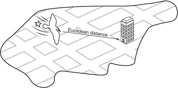
Euclidean distance
As we learn in geometry, the shortest path between two points is a straight line. It makes sense, then, that a straight-line heuristic will always be admissible for the maze-solving problem. The Euclidean distance, derived from the Pythagorean theorem, states that distance = √((difference in x)2 + (difference in y)2). For our mazes, the difference in x is equivalent to the difference in columns between two maze locations, and the difference in y is equivalent to the difference in rows. Note that we are implementing this back in maze.py.
Listing 2.26. maze.py continued
def euclidean_distance(goal: MazeLocation) -> Callable[[MazeLocation],
     float]:
    def distance(ml: MazeLocation) -> float:
        xdist: int = ml.column - goal.column
        ydist: int = ml.row - goal.row
        return sqrt((xdist * xdist) + (ydist * ydist))
    return distance
euclidean_distance() is a function that returns another function. Languages like Python that support first-class functions enable this interesting pattern. distance() captures the goal MazeLocation that euclidean_distance() is passed. Capturing means that distance() can refer to this variable every time it’s called (permanently). The function it returns makes use of goal to do its calculations. This pattern enables the creation of a function that requires fewer parameters. The returned distance() function takes just the start maze location as an argument and permanently “knows” the goal.
Figure 2.6 illustrates Euclidean distance within the context of a grid, like the streets of Manhattan.
Figure 2.6. Euclidean distance is the length of a straight line from the starting point to the goal.
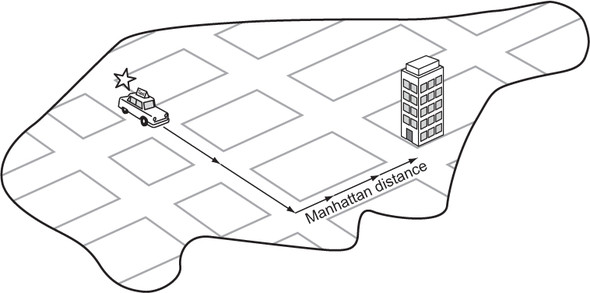
Manhattan distance
Euclidean distance is great, but for our particular problem (a maze in which you can move only in one of four directions) we can do even better. The Manhattan distance is derived from navigating the streets of Manhattan, the most famous of New York City’s boroughs, which is laid out in a grid pattern. To get from anywhere to anywhere in Manhattan, one needs to walk a certain number of horizontal blocks and a certain number of vertical blocks. (There are almost no diagonal streets in Manhattan.) The Manhattan distance is derived by simply finding the difference in rows between two maze locations and summing it with the difference in columns. Figure 2.7 illustrates Manhattan distance.
Listing 2.27. maze.py continued
def manhattan_distance(goal: MazeLocation) -> Callable[[MazeLocation],
     float]:
    def distance(ml: MazeLocation) -> float:
        xdist: int = abs(ml.column - goal.column)
        ydist: int = abs(ml.row - goal.row)
        return (xdist + ydist)
    return distance
Figure 2.7. In Manhattan distance, there are no diagonals. The path must be along parallel or perpendicular lines.
Because this heuristic more accurately follows the actuality of navigating our mazes (moving vertically and horizontally instead of in diagonal straight lines), it comes closer to the actual distance between any maze location and the goal than Euclidean distance does. Therefore, when an A* search is coupled with Manhattan distance, it will result in searching through fewer states than when an A* search is coupled with Euclidean distance for our mazes. Solution paths will still be optimal, because Manhattan distance is admissible (never overestimates distance) for mazes in which only four directions of movement are allowed.
The A* algorithm
To go from BFS to A* search, we need to make several small modifications. The first is changing the frontier from a queue to a priority queue. This way, the frontier will pop nodes with the lowest f(n). The second is changing the explored set to a dictionary. A dictionary will allow us to keep track of the lowest cost (g(n)) of each node we may visit. With the heuristic function now at play, it is possible some nodes may be visited twice if the heuristic is inconsistent. If the node found through the new direction has a lower cost to get to than the prior time we visited it, we will prefer the new route.
For the sake of simplicity, the function astar() does not take a cost-calculation function as a parameter. Instead, we just consider every hop in our maze to be a cost of 1. Each new Node gets assigned a cost based on this simple formula, as well as a heuristic score using a new function passed as a parameter to the search function called heuristic(). Other than these changes, astar() is remarkably similar to bfs(). Examine them side by side for comparison.
Listing 2.28. generic_search.py
def astar(initial: T, goal_test: Callable[[T], bool], successors:
     Callable[[T], List[T]], heuristic: Callable[[T], float]) ->
     Optional[Node[T]]:
    # frontier is where we've yet to go
    frontier: PriorityQueue[Node[T]] = PriorityQueue()
    frontier.push(Node(initial, None, 0.0, heuristic(initial)))
    # explored is where we've been
    explored: Dict[T, float] = {initial: 0.0}

    # keep going while there is more to explore
    while not frontier.empty:
        current_node: Node[T] = frontier.pop()
        current_state: T = current_node.state
        # if we found the goal, we're done
        if goal_test(current_state):
            return current_node
        # check where we can go next and haven't explored
        for child in successors(current_state):
            new_cost: float = current_node.cost + 1  # 1 assumes a grid, need
     a cost function for more sophisticated apps

            if child not in explored or explored[child] > new_cost:
                explored[child] = new_cost
                frontier.push(Node(child, current_node, new_cost,
     heuristic(child)))
    return None  # went through everything and never found goal
Congratulations. If you have followed along this far, you have learned not only how to solve a maze, but also some generic search functions that you can use in many different search applications. DFS and BFS are suitable for many smaller data sets and state spaces where performance is not critical. In some situations, DFS will outperform BFS, but BFS has the advantage of always delivering an optimal path. Interestingly, BFS and DFS have identical implementations, only differentiated by the use of a queue instead of a stack for the frontier. The slightly more complicated A* search, coupled with a good, consistent, admissible heuristic, not only delivers optimal paths, but also far outperforms BFS. And because all three of these functions were implemented generically, using them on nearly any search space is just an import generic_search away.
Go ahead and try out astar() with the same maze in maze.py’s testing section.
Listing 2.29. maze.py continued
# Test A*
distance: Callable[[MazeLocation], float] = manhattan_distance(m.goal)
solution3: Optional[Node[MazeLocation]] = astar(m.start, m.goal_test,
     m.successors, distance)
if solution3 is None:
    print("No solution found using A*!")
else:
    path3: List[MazeLocation] = node_to_path(solution3)
    m.mark(path3)
    print(m)
The output will interestingly be a little different from bfs(), even though both bfs() and astar() are finding optimal paths (equivalent in length). Due to its heuristic, astar() immediately drives through a diagonal toward the goal. It will ultimately search fewer states than bfs(), resulting in better performance. Add a state count to each if you want to prove this to yourself.
S**  X X
 X**
   *   X
 XX*     X
  X*
  X**X
 X  ****
       *
     X * X
       **G
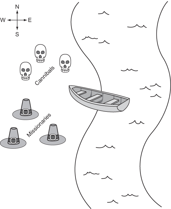
2.3. Missionaries and cannibals
Three missionaries and three cannibals are on the west bank of a river. They have a canoe that can hold two people, and they all must cross to the east bank of the river. There may never be more cannibals than missionaries on either side of the river, or the cannibals will eat the missionaries. Further, the canoe must have at least one person on board to cross the river. What sequence of crossings will successfully take the entire party across the river? Figure 2.8 illustrates the problem.
Figure 2.8. The missionaries and cannibals must use their single canoe to take everyone across the river from west to east. If the cannibals ever outnumber the missionaries, they will eat them.
2.3.1. Representing the problem
We will represent the problem by having a structure that keeps track of the west bank. How many missionaries and cannibals are on the west bank? Is the boat on the west bank? Once we have this knowledge, we can figure out what is on the east bank, because anything not on the west bank is on the east bank.
First, we will create a little convenience variable for keeping track of the maximum number of missionaries or cannibals. Then we will define the main class.
Listing 2.30. missionaries.py
from __future__ import annotations
from typing import List, Optional
from generic_search import bfs, Node, node_to_path

MAX_NUM: int = 3


class MCState:
    def __init__(self, missionaries: int, cannibals: int, boat: bool) ->
     None:
        self.wm: int = missionaries # west bank missionaries
        self.wc: int = cannibals # west bank cannibals
        self.em: int = MAX_NUM - self.wm  # east bank missionaries
        self.ec: int = MAX_NUM - self.wc  # east bank cannibals
        self.boat: bool = boat

    def __str__(self) -> str:
        return ("On the west bank there are {} missionaries and {}
     cannibals.\n"
                "On the east bank there are {} missionaries and {}
     cannibals.\n"
                "The boat is on the {} bank.")\
            .format(self.wm, self.wc, self.em, self.ec, ("west" if self.boat
     else "east"))
The class MCState initializes itself based on the number of missionaries and cannibals on the west bank as well as the location of the boat. It also knows how to pretty-print itself, which will be valuable later when displaying the solution to the problem.
Working within the confines of our existing search functions means that we must define a function for testing whether a state is the goal state and a function for finding the successors from any state. The goal test function, as in the maze-solving problem, is quite simple. The goal is simply when we reach a legal state that has all of the missionaries and cannibals on the east bank. We add it as a method to MCState.
Listing 2.31. missionaries.py continued
def goal_test(self) -> bool:
    return self.is_legal and self.em == MAX_NUM and self.ec == MAX_NUM
To create a successors function, it is necessary to go through all of the possible moves that can be made from one bank to another and then check if each of those moves will result in a legal state. Recall that a legal state is one in which cannibals do not outnumber missionaries on either bank. To determine this, we can define a convenience property (as a method on MCState) that checks if a state is legal.
Listing 2.32. missionaries.py continued
@property
def is_legal(self) -> bool:
    if self.wm < self.wc and self.wm > 0:
        return False
    if self.em < self.ec and self.em > 0:
        return False
    return True
The actual successors function is a bit verbose, for the sake of clarity. It tries adding every possible combination of one or two people moving across the river from the bank where the canoe currently resides. Once it has added all possible moves, it filters for the ones that are actually legal via a list comprehension. Once again, this is a method on MCState.
Listing 2.33. missionaries.py continued
def successors(self) -> List[MCState]:
    sucs: List[MCState] = []
    if self.boat: # boat on west bank
        if self.wm > 1:
            sucs.append(MCState(self.wm - 2, self.wc, not self.boat))
        if self.wm > 0:
            sucs.append(MCState(self.wm - 1, self.wc, not self.boat))
        if self.wc > 1:
            sucs.append(MCState(self.wm, self.wc - 2, not self.boat))
        if self.wc > 0:
            sucs.append(MCState(self.wm, self.wc - 1, not self.boat))
        if (self.wc > 0) and (self.wm > 0):
            sucs.append(MCState(self.wm - 1, self.wc - 1, not self.boat))
    else: # boat on east bank
        if self.em > 1:
            sucs.append(MCState(self.wm + 2, self.wc, not self.boat))
        if self.em > 0:
            sucs.append(MCState(self.wm + 1, self.wc, not self.boat))
        if self.ec > 1:
            sucs.append(MCState(self.wm, self.wc + 2, not self.boat))
        if self.ec > 0:
            sucs.append(MCState(self.wm, self.wc + 1, not self.boat))
        if (self.ec > 0) and (self.em > 0):
            sucs.append(MCState(self.wm + 1, self.wc + 1, not self.boat))
    return [x for x in sucs if x.is_legal]
2.3.2. Solving
We now have all of the ingredients in place to solve the problem. Recall that when we solve a problem using the search functions bfs(), dfs(), and astar(), we get back a Node that ultimately we convert using node_to_path() into a list of states that leads to a solution. What we still need is a way to convert that list into a comprehensible printed sequence of steps to solve the missionaries and cannibals problem.
The function display_solution() converts a solution path into printed output—a human-readable solution to the problem. It works by iterating through all of the states in the solution path while keeping track of the last state as well. It looks at the difference between the last state and the state it is currently iterating on to find out how many missionaries and cannibals moved across the river and in which direction.
Listing 2.34. missionaries.py continued
def display_solution(path: List[MCState]):
    if len(path) == 0: # sanity check
        return
    old_state: MCState = path[0]
    print(old_state)
    for current_state in path[1:]:
        if current_state.boat:
            print("{} missionaries and {} cannibals moved from the east bank
     to the west bank.\n"
                  .format(old_state.em - current_state.em, old_state.ec -
     current_state.ec))
        else:
            print("{} missionaries and {} cannibals moved from the west bank
     to the east bank.\n"
                  .format(old_state.wm - current_state.wm, old_state.wc -
     current_state.wc))
        print(current_state)
        old_state = current_state
The display_solution() function takes advantage of the fact that MCState knows how to pretty-print a nice summary of itself via __str__().
The last thing we need to do is actually solve the missionaries-and-cannibals problem. To do so we can conveniently reuse a search function that we have already implemented, because we implemented them generically. This solution uses bfs() (because using dfs() would require marking referentially different states with the same value as equal, and astar() would require a heuristic).
Listing 2.35. missionaries.py continued
if __name__ == "__main__":
    start: MCState = MCState(MAX_NUM, MAX_NUM, True)
    solution: Optional[Node[MCState]] = bfs(start, MCState.goal_test,
     MCState.successors)
    if solution is None:
        print("No solution found!")
    else:
        path: List[MCState] = node_to_path(solution)
        display_solution(path)
It is great to see how flexible our generic search functions can be. They can easily be adapted for solving a diverse set of problems. You should see output something like the following (abridged):
On the west bank there are 3 missionaries and 3 cannibals.
On the east bank there are 0 missionaries and 0 cannibals.
The boast is on the west bank.
0 missionaries and 2 cannibals moved from the west bank to the east bank.

On the west bank there are 3 missionaries and 1 cannibals.
On the east bank there are 0 missionaries and 2 cannibals.
The boast is on the east bank.
0 missionaries and 1 cannibals moved from the east bank to the west bank.

...

On the west bank there are 0 missionaries and 0 cannibals.
On the east bank there are 3 missionaries and 3 cannibals.
The boast is on the east bank.
2.4. Real-world applications
Search plays some role in all useful software. In some cases, it is the central element (Google Search, Spotlight, Lucene); in others, it is the basis for using the structures that underlie data storage. Knowing the correct search algorithm to apply to a data structure is essential for performance. For example, it would be very costly to use linear search, instead of binary search, on a sorted data structure.
A* is one of the most widely deployed path-finding algorithms. It is only beaten by algorithms that do precalculation in the search space. For a blind search, A* is yet to be reliably beaten in all scenarios, and this has made it an essential component of everything from route planning to figuring out the shortest way to parse a programming language. Most directions-providing map software (think Google Maps) uses Dijkstra’s algorithm (which A* is a variant of) to navigate. (There is more about Dijkstra’s algorithm in chapter 4.) Whenever an AI character in a game is finding the shortest path from one end of the world to the other without human intervention, it is probably using A*.
Breadth-first search and depth-first search are often the basis for more complex search algorithms like uniform-cost search and backtracking search (which you will see in the next chapter). Breadth-first search is often a sufficient technique for finding the shortest path in a fairly small graph. But due to its similarity to A*, it is easy to swap out for A* if a good heuristic exists for a larger graph.
2.5. Exercises
- Show the performance advantage of binary search over linear search by creating a list of one million numbers and timing how long it takes the linear_contains() and binary_contains() functions defined in this chapter to find various numbers in the list.
- Add a counter to dfs(), bfs(), and astar() to see how many states each searches through for the same maze. Find the counts for 100 different mazes to get statistically significant results.
- Find a solution to the missionaries-and-cannibals problem for a different number of starting missionaries and cannibals. Hint: you may need to add overrides of the __eq__() and __hash__() methods to MCState.