Chapter 1. Small problems
To get started, we will explore some simple problems that can be solved with no more than a few relatively short functions. Although these problems are small, they will still allow us to explore some interesting problem-solving techniques. Think of them as a good warm-up.
1.1. The Fibonacci sequence
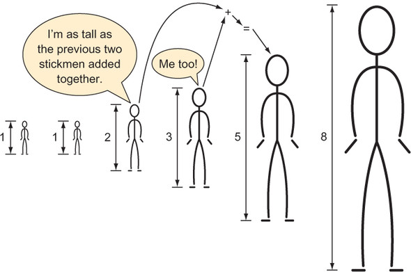
The Fibonacci sequence is a sequence of numbers such that any number, except for the first and second, is the sum of the previous two:
0, 1, 1, 2, 3, 5, 8, 13, 21...
The value of the first Fibonacci number in the sequence is 0. The value of the fourth Fibonacci number is 2. It follows that to get the value of any Fibonacci number, n, in the sequence, one can use the formula
fib(n) = fib(n - 1) + fib(n - 2)
1.1.1. A first recursive attempt
The preceding formula for computing a number in the Fibonacci sequence (illustrated in figure 1.1) is a form of pseudocode that can be trivially translated into a recursive Python function. (A recursive function is a function that calls itself.) This mechanical translation will serve as our first attempt at writing a function to return a given value of the Fibonacci sequence.
Listing 1.1. fib1.py
def fib1(n: int) -> int:
    return fib1(n - 1) + fib1(n - 2)
Figure 1.1. The height of each stickman is the previous two stickmen’s heights added together.
Let’s try to run this function by calling it with a value.
Listing 1.2. fib1.py continued
if __name__ == "__main__":
    print(fib1(5))
Uh-oh! If we try to run fib1.py, we generate an error:
RecursionError: maximum recursion depth exceeded
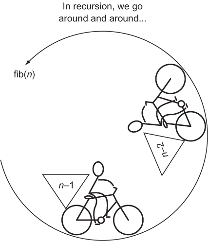
The issue is that fib1() will run forever without returning a final result. Every call to fib1() results in another two calls of fib1() with no end in sight. We call such a circumstance infinite recursion (see figure 1.2), and it is analogous to an infinite loop.
Figure 1.2. The recursive function fib(n) calls itself with the arguments n-2 and n-1.
1.1.2. Utilizing base cases
Notice that until you run fib1(), there is no indication from your Python environment that there is anything wrong with it. It is the duty of the programmer to avoid infinite recursion, not the compiler or the interpreter. The reason for the infinite recursion is that we never specified a base case. In a recursive function, a base case serves as a stopping point.
In the case of the Fibonacci function, we have natural base cases in the form of the special first two sequence values, 0 and 1. Neither 0 nor 1 is the sum of the previous two numbers in the sequence. Instead, they are the special first two values. Let’s try specifying them as base cases.
Listing 1.3. fib2.py
def fib2(n: int) -> int:
    if n < 2:  # base case
        return n
    return fib2(n - 2) + fib2(n - 1)  # recursive case
Note
The fib2() version of the Fibonacci function returns 0 as the zeroth number (fib2(0)), rather than the first number, as in our original proposition. In a programming context, this kind of makes sense because we are used to sequences starting with a zeroth element.
fib2() can be called successfully and will return correct results. Try calling it with some small values.
Listing 1.4. fib2.py continued
if __name__ == "__main__":
    print(fib2(5))
    print(fib2(10))
Do not try calling fib2(50). It will never finish executing! Why? Every call to fib2() results in two more calls to fib2() by way of the recursive calls fib2(n - 1) and fib2(n - 2) (see figure 1.3). In other words, the call tree grows exponentially. For example, a call of fib2(4) results in this entire set of calls:
fib2(4) -> fib2(3), fib2(2)
fib2(3) -> fib2(2), fib2(1)
fib2(2) -> fib2(1), fib2(0)
fib2(2) -> fib2(1), fib2(0)
fib2(1) -> 1
fib2(1) -> 1
fib2(1) -> 1
fib2(0) -> 0
fib2(0) -> 0
Figure 1.3. Every non-base-case call of fib2() results in two more calls of fib2().
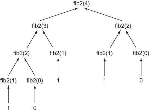
If you count them (and as you will see if you add some print calls), there are 9 calls to fib2() just to compute the 4th element! It gets worse. There are 15 calls required to compute element 5, 177 calls to compute element 10, and 21,891 calls to compute element 20. We can do better.
1.1.3. Memoization to the rescue
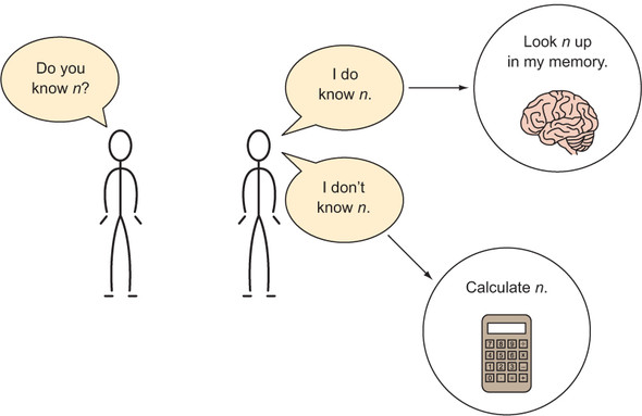
Memoization is a technique in which you store the results of computational tasks when they are completed so that when you need them again, you can look them up instead of needing to compute them a second (or millionth) time (see figure 1.4).[1]
Donald Michie, a famous British computer scientist, coined the term memoization. Donald Michie, Memo functions: a language feature with “rote-learning” properties (Edinburgh University, Department of Machine Intelligence and Perception, 1967).
Figure 1.4. The human memoization machine
Let’s create a new version of the Fibonacci function that utilizes a Python dictionary for memoization purposes.
Listing 1.5. fib3.py
from typing import Dict
memo: Dict[int, int] = {0: 0, 1: 1}  # our base cases

def fib3(n: int) -> int:
    if n not in memo:
        memo[n] = fib3(n - 1) + fib3(n - 2)  # memoization
    return memo[n]
You can now safely call fib3(50).
Listing 1.6. fib3.py continued
if __name__ == "__main__":
    print(fib3(5))
    print(fib3(50))
A call to fib3(20) will result in just 39 calls of fib3() as opposed to the 21,891 of fib2() resulting from the call fib2(20). memo is prefilled with the earlier base cases of 0 and 1, saving fib3() from the complexity of another if statement.
1.1.4. Automatic memoization
fib3() can be further simplified. Python has a built-in decorator for memoizing any function automagically. In fib4(), the decorator @functools.lru_cache() is used with the same exact code as we used in fib2(). Each time fib4() is executed with a novel argument, the decorator causes the return value to be cached. Upon future calls of fib4() with the same argument, the previous return value of fib4() for that argument is retrieved from the cache and returned.
Listing 1.7. fib4.py
from functools import lru_cache

@lru_cache(maxsize=None)
def fib4(n: int) -> int:  # same definition as fib2()
    if n < 2:  # base case
        return n
    return fib4(n - 2) + fib4(n - 1)  # recursive case

if __name__ == "__main__":
    print(fib4(5))
    print(fib4(50))
Note that we are able to calculate fib4(50) instantly, even though the body of the Fibonacci function is the same as that in fib2(). @lru_cache’s maxsize property indicates how many of the most recent calls of the function it is decorating should be cached. Setting it to None indicates that there is no limit.
1.1.5. Keep it simple, Fibonacci
There is an even more performant option. We can solve Fibonacci with an old-fashioned iterative approach.
Listing 1.8. fib5.py
def fib5(n: int) -> int:
    if n == 0: return n  # special case
    last: int = 0  # initially set to fib(0)
    next: int = 1  # initially set to fib(1)
    for _ in range(1, n):
        last, next = next, last + next
    return next

if __name__ == "__main__":
    print(fib5(5))
    print(fib5(50))
Warning
The body of the for loop in fib5() uses tuple unpacking in perhaps a bit of an overly clever way. Some may feel that it sacrifices readability for conciseness. Others may find the conciseness in and of itself more readable. The gist is, last is being set to the previous value of next, and next is being set to the previous value of last plus the previous value of next. This avoids the creation of a temporary variable to hold the old value of next after last is updated but before next is updated. Using tuple unpacking in this fashion for some kind of variable swap is common in Python.
With this approach, the body of the for loop will run a maximum of n - 1 times. In other words, this is the most efficient version yet. Compare 19 runs of the for loop body to 21,891 recursive calls of fib2() for the 20th Fibonacci number. That could make a serious difference in a real-world application!
In the recursive solutions, we worked backward. In this iterative solution, we work forward. Sometimes recursion is the most intuitive way to solve a problem. For example, the meat of fib1() and fib2() is pretty much a mechanical translation of the original Fibonacci formula. However, naive recursive solutions can also come with significant performance costs. Remember, any problem that can be solved recursively can also be solved iteratively.
1.1.6. Generating Fibonacci numbers with a generator
So far, we have written functions that output a single value in the Fibonacci sequence. What if we want to output the entire sequence up to some value instead? It is easy to convert fib5() into a Python generator using the yield statement. When the generator is iterated, each iteration will spew a value from the Fibonacci sequence using a yield statement.
Listing 1.9. fib6.py
from typing import Generator

def fib6(n: int) -> Generator[int, None, None]:
    yield 0  # special case
    if n > 0: yield 1  # special case
    last: int = 0  # initially set to fib(0)
    next: int = 1  # initially set to fib(1)
    for _ in range(1, n):
        last, next = next, last + next
        yield next  # main generation step

if __name__ == "__main__":
    for i in fib6(50):
        print(i)
If you run fib6.py, you will see 51 numbers in the Fibonacci sequence printed. For each iteration of the for loop for i in fib6(50):, fib6() runs through to a yield statement. If the end of the function is reached and there are no more yield statements, the loop finishes iterating.
1.2. Trivial compression
Saving space (virtual or real) is often important. It is more efficient to use less space, and it can save money. If you are renting an apartment that is bigger than you need for your things and family, you could “downsize” to a smaller place that is less expensive. If you are paying by the byte to store your data on a server, you may want to compress it so that its storage costs you less. Compression is the act of taking data and encoding it (changing its form) in such a way that it takes up less space. Decompression is reversing the process, returning the data to its original form.
If it is more storage-efficient to compress data, then why is all data not compressed? There is a tradeoff between time and space. It takes time to compress a piece of data and to decompress it back into its original form. Therefore, data compression only makes sense in situations where small size is prioritized over fast execution. Think of large files being transmitted over the internet. Compressing them makes sense because it will take longer to transfer the files than it will to decompress them once received. Further, the time taken to compress the files for their storage on the original server only needs to be accounted for once.
The easiest data compression wins come about when you realize that data storage types use more bits than are strictly required for their contents. For instance, thinking low-level, if an unsigned integer that will never exceed 65,535 is being stored as a 64-bit unsigned integer in memory, it is being stored inefficiently. It could instead be stored as a 16-bit unsigned integer. This would reduce the space consumption for the actual number by 75% (16 bits instead of 64 bits). If millions of such numbers are being stored inefficiently, it can add up to megabytes of wasted space.
In Python, sometimes for the sake of simplicity (which is a legitimate goal, of course), the developer is shielded from thinking in bits. There is no 64-bit unsigned integer type, and there is no 16-bit unsigned integer type. There is just a single int type that can store numbers of arbitrary precision. The function sys.getsizeof() can help you find out how many bytes of memory your Python objects are consuming. But due to the inherent overhead of the Python object system, there is no way to create an int that takes up less than 28 bytes (224 bits) in Python 3.7. A single int can be extended one bit at a time (as we will do in this example), but it consumes a minimum of 28 bytes.
Note
If you are a little rusty regarding binary, recall that a bit is a single value that is either a 1 or a 0. A sequence of 1s and 0s is read in base 2 to represent a number. For the purposes of this section, you do not need to do any math in base 2, but you do need to understand that the number of bits that a type stores determines how many different values it can represent. For example, 1 bit can represent 2 values (0 or 1), 2 bits can represent 4 values (00, 01, 10, 11), 3 bits can represent 8 values, and so on.
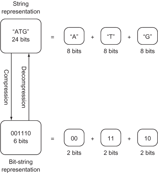
If the number of possible different values that a type is meant to represent is less than the number of values that the bits being used to store it can represent, it can likely be more efficiently stored. Consider the nucleotides that form a gene in DNA.[2] Each nucleotide can only be one of four values: A, C, G, or T. (There will be more about this in chapter 2.) Yet if the gene is stored as a str, which can be thought of as a collection of Unicode characters, each nucleotide will be represented by a character, which generally requires 8 bits of storage. In binary, just 2 bits are needed to store a type with four possible values: 00, 01, 10, and 11 are the four different values that can be represented by 2 bits. If A is assigned 00, C is assigned 01, G is assigned 10, and T is assigned 11, the storage required for a string of nucleotides can be reduced by 75% (from 8 bits to 2 bits per nucleotide).
This example is inspired by Algorithms, 4th Edition, by Robert Sedgewick and Kevin Wayne (Addison-Wesley Professional, 2011), page 819.
Instead of storing our nucleotides as a str, they can be stored as a bit string (see figure 1.5). A bit string is exactly what it sounds like: an arbitrary-length sequence of 1s and 0s. Unfortunately, the Python standard library contains no off-the-shelf construct for working with bit strings of arbitrary length. The following code converts a str composed of As, Cs, Gs, and Ts into a string of bits and back again. The string of bits is stored within an int. Because the int type in Python can be of any length, it can be used as a bit string of any length. To convert back into a str, we will implement the Python __str__() special method.
Figure 1.5. Compressing a str representing a gene into a 2-bit-per-nucleotide bit string
Listing 1.10. trivial_compression.py
class CompressedGene:
    def __init__(self, gene: str) -> None:
        self._compress(gene)
A CompressedGene is provided a str of characters representing the nucleotides in a gene, and it internally stores the sequence of nucleotides as a bit string. The __init__() method’s main responsibility is to initialize the bit-string construct with the appropriate data. __init__() calls _compress() to do the dirty work of actually converting the provided str of nucleotides into a bit string.
Note that _compress() starts with an underscore. Python has no concept of truly private methods or variables. (All variables and methods can be accessed through reflection; there’s no strict enforcement of privacy.) A leading underscore is used as a convention to indicate that the implementation of a method should not be relied on by actors outside of the class. (It is subject to change and should be treated as private.)
Tip
If you start a method or instance variable name in a class with two leading underscores, Python will “name mangle” it, changing its implementation name with a salt and not making it easily discoverable by other classes. We use one underscore in this book to indicate a “private” variable or method, but you may wish to use two if you really want to emphasize that something is private. For more on naming in Python, check out the section “Descriptive Naming Styles” from PEP 8: http://mng.bz/NA52.
Next, let’s look at how we can actually perform the compression.
Listing 1.11. trivial_compression.py continued
def _compress(self, gene: str) -> None:
    self.bit_string: int = 1  # start with sentinel
    for nucleotide in gene.upper():
        self.bit_string <<= 2  # shift left two bits
        if nucleotide == "A":  # change last two bits to 00
            self.bit_string |= 0b00
        elif nucleotide == "C":  # change last two bits to 01
            self.bit_string |= 0b01
        elif nucleotide == "G":  # change last two bits to 10
            self.bit_string |= 0b10
        elif nucleotide == "T":  # change last two bits to 11
            self.bit_string |= 0b11
        else:
            raise ValueError("Invalid Nucleotide:{}".format(nucleotide))
The _compress()method looks at each character in the str of nucleotides sequentially. When it sees an A, it adds 00 to the bit string. When it sees a C, it adds 01, and so on. Remember that two bits are needed for each nucleotide. As a result, before we add each new nucleotide, we shift the bit string two bits to the left (self.bit_string <<= 2).
Every nucleotide is added using an “or” operation (|). After the left shift, two 0s are added to the right side of the bit string. In bitwise operations, “ORing” (for example, self.bit_string |= 0b10) 0s with any other value results in the other value replacing the 0s. In other words, we continually add two new bits to the right side of the bit string. The two bits that are added are determined by the type of the nucleotide.
Finally, we will implement decompression and the special __str__() method that uses it.
Listing 1.12. trivial_compression.py continued
def decompress(self) -> str:
    gene: str = ""
    for i in range(0, self.bit_string.bit_length() - 1, 2):  # - 1 to exclude
     sentinel
        bits: int = self.bit_string >> i & 0b11  # get just 2 relevant bits
        if bits == 0b00:  # A
            gene += "A"
        elif bits == 0b01:  # C
            gene += "C"
        elif bits == 0b10:  # G
            gene += "G"
        elif bits == 0b11:  # T
            gene += "T"
        else:
            raise ValueError("Invalid bits:{}".format(bits))
    return gene[::-1]  # [::-1] reverses string by slicing backward

def __str__(self) -> str:  # string representation for pretty printing
    return self.decompress()
decompress() reads two bits from the bit string at a time, and it uses those two bits to determine which character to add to the end of the str representation of the gene. Because the bits are being read backward, compared to the order they were compressed in (right to left instead of left to right), the str representation is ultimately reversed (using the slicing notation for reversal [::-1]). Finally, note how the convenient int method bit_length() aided in the development of decompress(). Let’s test it out.
Listing 1.13. trivial_compression.py continued
if __name__ == "__main__":
    from sys import getsizeof
    original: str =
     "TAGGGATTAACCGTTATATATATATAGCCATGGATCGATTATATAGGGATTAACCGTTATATATATATAGC
     CATGGATCGATTATA" * 100
    print("original is {} bytes".format(getsizeof(original)))
    compressed: CompressedGene = CompressedGene(original)  # compress
    print("compressed is {} bytes".format(getsizeof(compressed.bit_string)))
    print(compressed)  # decompress
    print("original and decompressed are the same: {}".format(original ==
     compressed.decompress()))
Using the sys.getsizeof() method, we can indicate in the output whether we did indeed save almost 75% of the memory cost of storing the gene through this compression scheme.
Listing 1.14. trivial_compression.py output
original is 8649 bytes
compressed is 2320 bytes
TAGGGATTAACC...
original and decompressed are the same: True
NOTE
In the CompressedGene class, we used if statements extensively to decide between a series of cases in both the compression and the decompression methods. Because Python has no switch statement, this is somewhat typical. What you will also see in Python sometimes is a high reliance on dictionaries in place of extensive if statements to deal with a set of cases. Imagine, for instance, a dictionary in which we could look up each nucleotide’s respective bits. This can sometimes be more readable, but it can come with a performance cost. Even though a dictionary lookup is technically O(1), the cost of running a hash function will sometimes mean a dictionary is less performant than a series of ifs. Whether this holds will depend on what a particular program’s if statements must evaluate to make their decision. You may want to run performance tests on both methods if you need to make a decision between ifs and dictionary lookup in a critical section of code.
1.3. Unbreakable encryption
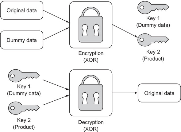
A one-time pad is a way of encrypting a piece of data by combining it with meaningless random dummy data in such a way that the original cannot be reconstituted without access to both the product and the dummy data. In essence, this leaves the encrypter with a key pair. One key is the product, and the other is the random dummy data. One key on its own is useless; only the combination of both keys can unlock the original data. When performed correctly, a one-time pad is a form of unbreakable encryption. Figure 1.6 shows the process.
Figure 1.6. A one-time pad results in two keys that can be separated and then recombined to re-create the original data.
1.3.1. Getting the data in order
In this example, we will encrypt a str using a one-time pad. One way of thinking about a Python 3 str is as a sequence of UTF-8 bytes (with UTF-8 being a Unicode character encoding). A str can be converted into a sequence of UTF-8 bytes (represented as the bytes type) through the encode() method. Likewise, a sequence of UTF-8 bytes can be converted back into a str using the decode() method on the bytes type.
There are three criteria that the dummy data used in a one-time pad encryption operation must meet for the resulting product to be unbreakable. The dummy data must be the same length as the original data, truly random, and completely secret. The first and third criteria are common sense. If the dummy data repeats because it is too short, there could be an observed pattern. If one of the keys is not truly secret (perhaps it is reused elsewhere or partially revealed), then an attacker has a clue. The second criteria poses a question all its own: can we produce truly random data? The answer for most computers is no.
In this example we will use the pseudo-random data generating function token_bytes() from the secrets module (first included in the standard library in Python 3.6). Our data will not be truly random, in the sense that the secrets package still is using a pseudo-random number generator behind the scenes, but it will be close enough for our purposes. Let’s generate a random key for use as dummy data.
Listing 1.15. unbreakable_encryption.py
from secrets import token_bytes
from typing import Tuple

def random_key(length: int) -> int:
    # generate length random bytes
    tb: bytes = token_bytes(length)
    # convert those bytes into a bit string and return it
    return int.from_bytes(tb, "big")
This function creates an int filled with length random bytes. The method int.from_bytes() is used to convert from bytes to int. How can multiple bytes be converted to a single integer? The answer lies in section 1.2. In that section, you learned that the int type can be of arbitrary size, and you saw how it can be used as a generic bit string. int is being used in the same way here. For example, the from_bytes() method will take 7 bytes (7 bytes * 8 bits = 56 bits) and convert them into a 56-bit integer. Why is this useful? Bitwise operations can be executed more easily and performantly on a single int (read “long bit string”) than on many individual bytes in a sequence. And we are about to use the bitwise operation XOR.
1.3.2. Encrypting and decrypting
How will the dummy data be combined with the original data that we want to encrypt? The XOR operation will serve this purpose. XOR is a logical bitwise (operates at the bit level) operation that returns true when one of its operands is true but returns false when both are true or neither is true. As you may have guessed, XOR stands for exclusive or.
In Python, the XOR operator is ^. In the context of the bits of binary numbers, XOR returns 1 for 0 ^ 1 and 1 ^ 0, but 0 for 0 ^ 0 and 1 ^ 1. If the bits of two numbers are combined using XOR, a helpful property is that the product can be recombined with either of the operands to produce the other operand:
A ^ B = C
C ^ B = A
C ^ A = B
This key insight forms the basis of one-time pad encryption. To form our product, we will simply XOR an int representing the bytes in our original str with a randomly generated int of the same bit length (as produced by random_key()). Our returned key pair will be the dummy data and the product.
Listing 1.16. unbreakable_encryption.py continued
def encrypt(original: str) -> Tuple[int, int]:
    original_bytes: bytes = original.encode()
    dummy: int = random_key(len(original_bytes))
    original_key: int = int.from_bytes(original_bytes, "big")
    encrypted: int = original_key ^ dummy  # XOR
    return dummy, encrypted
Note
int.from_bytes() is being passed two arguments. The first is the bytes that we want to convert into an int. The second is the endianness of those bytes ("big"). Endianness refers to the byte-ordering used to store data. Does the most significant byte come first, or does the least significant byte come first? In our case, it does not matter as long as we use the same ordering both when we encrypt and decrypt, because we are actually only manipulating the data at the individual bit level. In other situations, when you are not controlling both ends of the encoding process, the ordering can absolutely matter, so be careful!
Decryption is simply a matter of recombining the key pair we generated with encrypt(). This is achieved once again by doing an XOR operation between each and every bit in the two keys. The ultimate output must be converted back to a str. First, the int is converted to bytes using int.to_bytes(). This method requires the number of bytes to be converted from the int. To get this number, we divide the bit length by eight (the number of bits in a byte). Finally, the bytes method decode() gives us back a str.
Listing 1.17. unbreakable_encryption.py continued
def decrypt(key1: int, key2: int) -> str:
    decrypted: int = key1 ^ key2  # XOR
    temp: bytes = decrypted.to_bytes((decrypted.bit_length()+ 7) // 8, "big")
    return temp.decode()
It was necessary to add 7 to the length of the decrypted data before using integer-division (//) to divide by 8 to ensure that we “round up,” to avoid an off-by-one error. If our one-time pad encryption truly works, we should be able to encrypt and decrypt the same Unicode string without issue.
Listing 1.18. unbreakable_encryption.py continued
if __name__ == "__main__":
    key1, key2 = encrypt("One Time Pad!")
    result: str = decrypt(key1, key2)
    print(result)
If your console outputs One Time Pad! then everything worked.
1.4. Calculating pi
The mathematically significant number pi (π or 3.14159...) can be derived using many formulas. One of the simplest is the Leibniz formula. It posits that the convergence of the following infinite series is equal to pi:
π = 4/1 - 4/3 + 4/5 - 4/7 + 4/9 - 4/11...
You will notice that the infinite series’ numerator remains 4 while the denominator increases by 2, and the operation on the terms alternates between addition and subtraction.
We can model the series in a straightforward way by translating pieces of the formula into variables in a function. The numerator can be a constant 4. The denominator can be a variable that begins at 1 and is incremented by 2. The operation can be represented as either -1 or 1 based on whether we are adding or subtracting. Finally, the variable pi is used in listing 1.19 to collect the sum of the series as the for loop proceeds.
Listing 1.19. calculating_pi.py
def calculate_pi(n_terms: int) -> float:
    numerator: float = 4.0
    denominator: float = 1.0
    operation: float = 1.0
    pi: float = 0.0
    for _ in range(n_terms):
        pi += operation * (numerator / denominator)
        denominator += 2.0
        operation *= -1.0
    return pi

if __name__ == "__main__":
    print(calculate_pi(1000000))
Tip
On most platforms, Python floats are 64-bit floating-point numbers (or double in C).
This function is an example of how rote conversion between formula and programmatic code can be both simple and effective in modeling or simulating an interesting concept. Rote conversion is a useful tool, but we must keep in mind that it is not necessarily the most efficient solution. Certainly, the Leibniz formula for pi can be implemented with more efficient or compact code.
Note
The more terms in the infinite series (the higher the value of n_terms when calculate_pi() is called), the more accurate the ultimate calculation of pi will be.
1.5. The Towers of Hanoi
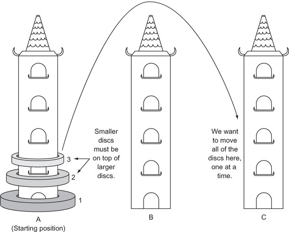
Three vertical pegs (henceforth “towers”) stand tall. We will label them A, B, and C. Doughnut-shaped discs are around tower A. The widest disc is at the bottom, and we will call it disc 1. The rest of the discs above disc 1 are labeled with increasing numerals and get progressively narrower. For instance, if we were to work with three discs, the widest disc, the one on the bottom, would be 1. The next widest disc, disc 2, would sit on top of disc 1. And finally, the narrowest disc, disc 3, would sit on top of disc 2. Our goal is to move all of the discs from tower A to tower C given the following constraints:
- Only one disc can be moved at a time.
- The topmost disc of any tower is the only one available for moving.
- A wider disc can never be atop a narrower disc.
Figure 1.7 summarizes the problem.
Figure 1.7. The challenge is to move the three discs, one at a time, from tower A to tower C. A larger disc may never be on top of a smaller disc.
1.5.1. Modeling the towers
A stack is a data structure that is modeled on the concept of Last-In-First-Out (LIFO). The last thing put into it is the first thing that comes out of it. The two most basic operations on a stack are push and pop. A push puts a new item into a stack, whereas a pop removes and returns the last item put in. We can easily model a stack in Python using a list as a backing store.
Listing 1.20. hanoi.py
from typing import TypeVar, Generic, List
T = TypeVar('T')

class Stack(Generic[T]):

    def __init__(self) -> None:
        self._container: List[T] = []

    def push(self, item: T) -> None:
        self._container.append(item)

    def pop(self) -> T:
        return self._container.pop()

    def __repr__(self) -> str:
        return repr(self._container)
Note
This Stack class implements __repr__() so that we can easily explore the contents of a tower. __repr__() is what will be output when print() is applied to a Stack.
Note
As was described in the introduction, this book utilizes type hints throughout. The import of Generic from the typing module enables Stack to be generic over a particular type in type hints. The arbitrary type T is defined in T = TypeVar('T'). T can be any type. When a type hint is later used for a Stack to solve the Hanoi problem, it is type-hinted as type Stack[int], which means T is filled in with type int. In other words, the stack is a stack of integers. If you are struggling with type hints, take a look at appendix C.
Stacks are perfect stand-ins for the towers in The Towers of Hanoi. When we want to put a disc onto a tower, we can just push it. When we want to move a disc from one tower to another, we can pop it from the first and push it onto the second.
Let’s define our towers as Stacks and fill the first tower with discs.
Listing 1.21. hanoi.py continued
num_discs: int = 3
tower_a: Stack[int] = Stack()
tower_b: Stack[int] = Stack()
tower_c: Stack[int] = Stack()
for i in range(1, num_discs + 1):
    tower_a.push(i)
1.5.2. Solving The Towers of Hanoi
How can The Towers of Hanoi be solved? Imagine we were only trying to move 1 disc. We would know how to do that, right? In fact, moving one disc is our base case for a recursive solution to The Towers of Hanoi. The recursive case is moving more than one disc. Therefore, the key insight is that we essentially have two scenarios we need to codify: moving one disc (the base case) and moving more than one disc (the recursive case).
Let’s look at a specific example to understand the recursive case. Say we have three discs (top, middle, and bottom) on tower A that we want to move to tower C. (It may help to sketch out the problem as you follow along.) We could first move the top disc to tower C. Then we could move the middle disc to tower B. Then we could move the top disc from tower C to tower B. Now we have the bottom disc still on tower A and the upper two discs on tower B. Essentially, we have now successfully moved two discs from one tower (A) to another tower (B). Moving the bottom disc from A to C is our base case (moving a single disc). Now we can move the two upper discs from B to C in the same procedure that we did from A to B. We move the top disc to A, the middle disc to C, and finally the top disc from A to C.
Tip
In a computer science classroom, it is not uncommon to see a little model of the towers built using dowels and plastic doughnuts. You can build your own model using three pencils and three pieces of paper. It may help you visualize the solution.
In our three-disc example, we had a simple base case of moving a single disc and a recursive case of moving all of the other discs (two in this case), using the third tower temporarily. We could break the recursive case into three steps:
- Move the upper n-1 discs from tower A to B (the temporary tower), using C as the in-between.
- Move the single lowest disc from A to C.
- Move the n-1 discs from tower B to C, using A as the in-between.
The amazing thing is that this recursive algorithm works not only for three discs, but for any number of discs. We will codify it as a function called hanoi() that is responsible for moving discs from one tower to another, given a third temporary tower.
Listing 1.22. hanoi.py continued
def hanoi(begin: Stack[int], end: Stack[int], temp: Stack[int], n: int) ->
     None:
    if n == 1:
        end.push(begin.pop())
    else:
        hanoi(begin, temp, end, n - 1)
        hanoi(begin, end, temp, 1)
        hanoi(temp, end, begin, n - 1)
After calling hanoi(), you should examine towers A, B, and C to verify that the discs were moved successfully.
Listing 1.23. hanoi.py continued
if __name__ == "__main__":
    hanoi(tower_a, tower_c, tower_b, num_discs)
    print(tower_a)
    print(tower_b)
    print(tower_c)
You will find that they were. In codifying the solution to The Towers of Hanoi, we did not necessarily need to understand every step required to move multiple discs from tower A to tower C. But we came to understand the general recursive algorithm for moving any number of discs, and we codified it, letting the computer do the rest. This is the power of formulating recursive solutions to problems: we often can think of solutions in an abstract manner without the drudgery of negotiating every individual action in our minds.
Incidentally, the hanoi() function will execute an exponential number of times as a function of the number of discs, which makes solving the problem for even 64 discs untenable. You can try it with various other numbers of discs by changing the num_discs variable. The exponentially increasing number of steps required as the number of discs increases is where the legend of The Towers of Hanoi comes from; you can read more about it in any number of sources. You may also be interested in reading more about the mathematics behind its recursive solution; see Carl Burch’s explanation in “About the Towers of Hanoi,” http://mng.bz/c1i2.
1.6. Real-world applications
The various techniques presented in this chapter (recursion, memoization, compression, and manipulation at the bit level) are so common in modern software development that it is impossible to imagine the world of computing without them. Although problems can be solved without them, it is often more logical or performant to solve problems with them.
Recursion, in particular, is at the heart of not just many algorithms, but even whole programming languages. In some functional programming languages, like Scheme and Haskell, recursion takes the place of the loops used in imperative languages. It is worth remembering, though, that anything accomplishable with a recursive technique is also accomplishable with an iterative technique.
Memoization has been applied successfully to speed up the work of parsers (programs that interpret languages). It is useful in all problems where the result of a recent calculation will likely be asked for again. Another application of memoization is in language runtimes. Some language runtimes (versions of Prolog, for instance) will store the results of function calls automatically (auto-memoization), so that the function need not execute the next time the same call is made. This is similar to how the @lru_cache() decorator in fib6() worked.
Compression has made an internet-connected world constrained by bandwidth more tolerable. The bit-string technique examined in section 1.2 is usable for real-world simple data types that have a limited number of possible values, for which even a byte is overkill. The majority of compression algorithms, however, operate by finding patterns or structures within a data set that allow for repeated information to be eliminated. They are significantly more complicated than what is covered in section 1.2.
One-time pads are not practical for general encryption. They require both the encrypter and the decrypter to have possession of one of the keys (the dummy data in our example) for the original data to be reconstructed, which is cumbersome and defeats the goal of most encryption schemes (keeping keys secret). But you may be interested to know that the name “one-time pad” comes from spies using real paper pads with dummy data on them to create encrypted communications during the Cold War.
These techniques are programmatic building blocks that other algorithms are built on top of. In future chapters you will see them applied liberally.
1.7. Exercises
- Write yet another function that solves for element n of the Fibonacci sequence, using a technique of your own design. Write unit tests that evaluate its correctness and performance relative to the other versions in this chapter.
- You saw how the simple int type in Python can be used to represent a bit string. Write an ergonomic wrapper around int that can be used generically as a sequence of bits (make it iterable and implement __getitem__()). Reimplement CompressedGene, using the wrapper.
- Write a solver for The Towers of Hanoi that works for any number of towers.
- Use a one-time pad to encrypt and decrypt images.