12.4 Performance
All things being equal, a fast operating system is better than a slow one. However, a fast unreliable operating system is not as good as a reliable slow one. Since complex optimizations often lead to bugs, it is important to use them sparingly. This notwithstanding, there are places where performance is critical and optimizations are worth the effort. In the following sections, we will look at some techniques that can be used to improve performance in places where that is called for.
12.4.1 Why Are Operating Systems Slow?
Before talking about optimization techniques, it is worth pointing out that the slowness of many operating systems is to a large extent self-inflicted. For example, older operating systems, such as MS-DOS and UNIX Version 7, booted within a few seconds. Modern UNIX systems and Windows can take many tens of seconds to boot, despite running on hardware that is 1000 times faster. The reason is that they are doing much more, wanted or not. A case in point. Plug and play makes it somewhat easier to install a new hardware device, but the price paid is that on every boot, the operating system has to go out and inspect all the hardware to see if there is anything new out there. This bus scan takes time.
An alternative (and, in the authors’ opinion, better) approach would be to scrap plug-and-play altogether and have an icon on the screen labeled ‘‘Install new hardware.’’ Upon installing a new hardware device, the user would click on it to start the bus scan, instead of doing it on every boot. The designers of current systems were well aware of this option, of course. They rejected it, basically, because they assumed that the users were too stupid to be able to do this correctly (although they would word it more kindly). This is only one example, but there are many more where the desire to make the system ‘‘user-friendly’’ slows the system down all the time for everyone.
Probably the biggest single thing system designers can do to improve performance is to be much more selective about adding new features. The question to ask is not whether some users like it, but whether it is worth the inevitable price in code size, speed, complexity, and reliability. Only if the advantages clearly outweigh the drawbacks should it be included. Programmers have a tendency to assume that code size and bug count will be 0 and speed will be infinite. Experience shows this view to be a wee bit optimistic.
Another factor that plays a role is product marketing. By the time version 4 or 5 of some product has hit the market, probably all the features that are actually useful have been included and most of the people who need the product already have it. To keep sales going, many manufacturers nevertheless continue to produce a steady stream of new versions, with more features, just so they can sell their existing customers upgrades. Adding new features just for the sake of adding new features may help sales but rarely helps performance. It almost never helps reliability.
12.4.2 What Should Be Optimized?
As a general rule, the first version of the system should be as straightforward as possible. The only optimizations should be things that are so obviously going to be a problem that they are unavoidable. Having a block cache for the file system is such an example. Once the system is up and running, careful measurements should be made to see where the time is really going. Based on these numbers, optimizations should be made where they will help most.
Here is a true story of where an optimization did more harm than good. One of the authors (AST) had a former student (who shall here remain nameless) who wrote the original MINIX mkfs program. This program lays down a fresh file system on a newly formatted disk. The student spent about 6 months optimizing it, including putting in disk caching. When he turned it in, it did not work and it required several additional months of debugging. This program typically runs on the hard disk once during the life of the computer, when the system is installed. It also runs once for each disk that is formatted. Each run takes about 2 sec. Even if the unoptimized version had taken 1 minute, it was a poor use of resources to spend so much time optimizing a program that is used so infrequently.
A slogan that has considerable applicability to performance optimization is
Good enough is good enough.
By this we mean that once the performance has achieved a reasonable level, it is probably not worth the effort and complexity to squeeze out the last few percent. If the scheduling algorithm is reasonably fair and keeps the CPU busy 90% of the time, it is doing its job. Devising a far more complex one that is 5% better is probably a bad idea. Similarly, if the page rate is low enough that it is not a bottleneck, jumping through hoops to get optimal performance is usually not worth it. Avoiding disaster is far more important than getting optimal performance, especially since what is optimal with one load may not be optimal with another.
Another concern is what to optimize when. Some programmers have a tendency to optimize to death whatever they develop, as soon as it is appears to work. The problem is that after optimization, the system may be less clean, making it harder to maintain and debug. Also, it makes it harder to adapt it, and perhaps do more fruitful optimization later. The problem is known as premature optimization. Donald Knuth, sometimes referred to as the father of the analysis of algorithms, once said that ‘‘premature optimization is the root of all evil.’’
12.4.3 Space-Time Trade-offs
One general approach to improving performance is to trade off time vs. space. It frequently occurs in computer science that there is a choice between an algorithm that uses little memory but is slow and an algorithm that uses much more memory but is faster. When making an important optimization, it is worth looking for algorithms that gain speed by using more memory or conversely save precious memory by doing more computation.
One technique that is sometimes helpful is to replace small procedures by macros. Using a macro eliminates the overhead that is associated with a procedure call. The gain is especially significant if the call occurs inside a loop. As an example, suppose we use bitmaps to keep track of resources and frequently need to know how many units are free in some portion of the bitmap. For this purpose we will need a procedure, bit count, that counts the number of 1 bits in a byte. The obvious procedure is given in Fig. 12-7(a). It loops over the bits in a byte, counting them one at a time. It is pretty simple and straightforward.
Figure 12-7
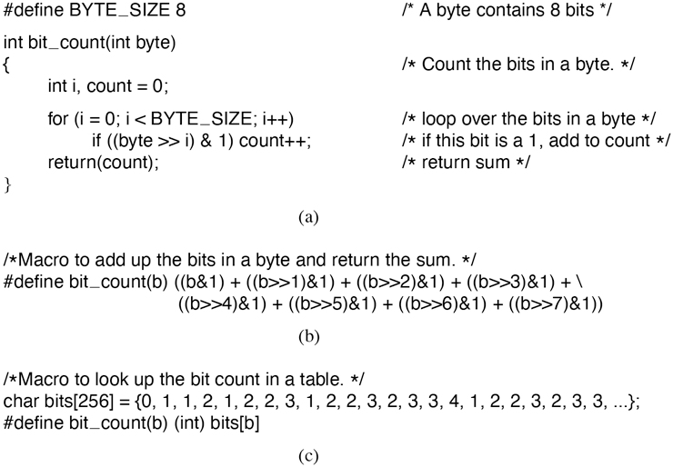
(a) A procedure for counting bits in a byte. (b) A macro to count the bits. (c) A macro that counts bits by table lookup.
This procedure has two sources of inefficiency. First, it must be called, stack space must be allocated for it, and it must return. Every procedure call has this overhead. Second, it contains a loop, and there is always some overhead associated with a loop.
A completely different approach is to use the macro of Fig. 12-7(b). It is an inline expression that computes the sum of the bits by successively shifting the argument, masking out everything but the low-order bit, and adding up the eight terms. The macro is hardly a work of art, but it appears in the code only once. When the macro is called, for example, by
sum = bit_count(table[i]);the macro call looks identical to the call of the procedure. Thus, other than one somewhat messy definition, the code does not look any worse in the macro case than in the procedure case, but it is much more efficient since it eliminates both the procedure-call overhead and the loop overhead.
We can take this example one step further. Why compute the bit count at all? Why not look it up in a table? After all, there are only 256 different bytes, each with a unique value between 0 and 8. We can declare a 256-entry table, bits, with each entry initialized (at compile time) to the bit count corresponding to that byte value. With this approach no computation at all is needed at run time, just one indexing operation. A macro to do the job is given in Fig. 12-7(c).
This is a clear example of trading computation time against memory. However, we could go still further. If the bit counts for whole 32-bit words are needed, using our bit_count macro, we need to perform four lookups per word. If we expand the table to 65,536 entries, we can suffice with two lookups per word, at the price of a much bigger table.
Looking answers up in tables can also be used in other ways. A well-known image-compression technique, GIF, uses table lookup to encode 24-bit RGB pixels. However, GIF only works on images with 256 or fewer colors. For each image to be compressed, a palette of 256 entries is constructed, each entry containing one 24-bit RGB value. The compressed image then consists of an 8-bit index for each pixel instead of a 24-bit color value, a gain of a factor of three. This idea is illustrated for a section of an image in Fig. 12-8. The original compressed image is shown in Fig. 12-8(a). Each value is a 24-bit value, with 8 bits for the intensity of red, green, and blue, respectively. The GIF image is shown in Fig. 12-8(b). Each value is an 8-bit index into the color palette. The color palette is stored as part of the image file, and is shown in Fig. 12-8(c). Actually, there is more to GIF, but the core idea is table lookup.
Figure 12-8
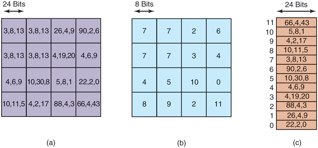
(a) Part of an uncompressed image with 24 bits per pixel. (b) The same part compressed with GIF, with 8 bits per pixel. (c) The color palette.
There is another way to reduce image size, and it illustrates a different tradeoff. PostScript is a programming language that can be used to describe images. (Actually, any programming language can describe images, but PostScript is tuned for this purpose.) Many printers have a PostScript interpreter built into them to be able to run PostScript programs sent to them.
For example, if there is a rectangular block of pixels all the same color in an image, a PostScript program for the image would carry instructions to place a rectangle at a certain location and fill it with a certain color. Only a handful of bits are needed to issue this command. When the image is received at the printer, an interpreter there must run the program to construct the image. Thus PostScript achieves data compression at the expense of more computation, a different trade-off than table lookup, but a valuable one when memory or bandwidth is scarce.
Other trade-offs often involve data structures. Doubly linked lists take up more memory than singly linked lists, but often allow faster access to items. Hash tables are even more wasteful of space, but faster still. In short, one of the main things to consider when optimizing a piece of code is whether using different data structures would make the best time-space trade-off.
12.4.4 Caching
A well-known technique for improving performance is caching. It is applicable whenever it is likely the same result will be needed multiple times. The general approach is to do the full work the first time, and then save the result in a cache. On subsequent attempts, the cache is first checked. If the result is there, it is used. Otherwise, the full work is done again.
We have already seen the use of caching within the file system to hold some number of recently used disk blocks, thus saving a disk read on each hit. However, caching can be used for many other purposes as well. For example, parsing path names is surprisingly expensive. Consider the UNIX example of Fig. 4-36 again. To look up /usr/ast/mbox requires the following disk accesses:
Read the i-node for the root directory (i-node 1).
Read the root directory (block 1).
Read the i-node for /usr (i-node 6).
Read the /usr directory (block 132).
Read the i-node for /usr/ast (i-node 26).
Read the /usr/ast directory (block 406).
aIt takes six disk accesses just to discover the i-node number of the file. Then the inode itself has to be read to discover the disk block numbers. If the file is smaller than the block size (e.g., 1024 bytes), it takes eight disk accesses to read the data.
Some systems optimize path-name parsing by caching (path, i-node) combinations. For the example of Fig. 4-36, the cache will certainly hold the first three entries of Fig. 12-9 after parsing /usr/ast/mbox. The last three entries come from parsing other paths.
Figure 12-9
| Path | I-node number |
|---|---|
| /usr | 6 |
| /usrlast | 26 |
| /usr/ast/mbox | 60 |
| /usr/ast/books | 92 |
| /usr/bal | 45 |
| /usr/bal/paper.ps | 85 |
Part of the i-node cache for Fig. 4-36.
When a path has to be looked up, the name parser first consults the cache and searches it for the longest substring present in the cache. For example, if the path /usr/ast/grants/erc is presented, the cache returns the fact that /usr/ast is i-node 26, so the search can start there, eliminating four disk accesses.
A problem with caching paths is that the mapping between file name and inode number is not fixed for all time. Suppose that the file /usr/ast/mbox is removed from the system and its i-node reused for a different file owned by a different user. Later, the file /usr/ast/mbox is created again, and this time it gets i-node 106. If nothing is done to prevent it, the cache entry will now be wrong and subsequent lookups will return the wrong i-node number. For this reason, when a file or directory is deleted, its cache entry and (if it is a directory) all the entries below it must be purged from the cache.
Disk blocks and path names are not the only items that are cacheable. I-nodes can be cached, too. If pop-up threads are used to handle interrupts, each one of them requires a stack and some additional machinery. These previously used threads can also be cached, since refurbishing a used one is easier than creating a new one from scratch (to avoid having to allocate memory). Just about anything that is hard to produce can be cached.
12.4.5 Hints
Cache entries are always correct. A cache search may fail, but if it finds an entry, that entry is guaranteed to be correct and can be used without further ado. In some systems, it is convenient to have a table of hints. These are suggestions about the solution, but they are not guaranteed to be correct. The called must verify the result itself.
A well-known example of hints are the URLs embedded on Web pages. Clicking on a link does not guarantee that the Web page pointed to is there. In fact, the page pointed to may have been removed 10 years ago. Thus the information on the pointing page is really only a hint.
Hints are also used in connection with remote files. The information in the hint tells something about the remote file, such as where it is located. However, the file may have moved or been deleted since the hint was recorded, so a check is always needed to see if it is correct.
12.4.6 Exploiting Locality
Processes and programs do not act at random. They exhibit a fair amount of locality in time and space, and this information can be exploited in various ways to improve performance. One well-known example of spatial locality is the fact that processes do not jump around at random within their address spaces. They tend to use a relatively small number of pages during a given time interval. The pages that a process is actively using can be noted as its working set, and the operating system can make sure that when the process is allowed to run, its working set is in memory, thus reducing the number of page faults.
The locality principle also holds for files. When a process has selected a particular working directory, it is likely that many of its future file references will be to files in that directory. By putting all the i-nodes and files for each directory close together on the disk, performance improvements can be obtained. This principle is what underlies the Berkeley Fast File System (McKusick et al., 1984).
Another area in which locality plays a role is in thread scheduling in multiprocessors. As we saw in Chap. 8, one way to schedule threads on a multiprocessor is to try to run each thread on the CPU it last used, in hopes that some of its memory blocks will still be in the memory cache.
12.4.7 Optimize the Common Case
It is frequently a good idea to distinguish between the most common case and the worst possible case and treat them differently. Often the code for the two is quite different. It is important to make the common case fast. For the worst case, if it occurs rarely, it is sufficient to make it correct.
As a first example, consider entering a critical region. Most of the time, the entry will succeed, especially if processes do not spend a lot of time inside critical regions. Windows takes advantage of this expectation by providing a WinAPI call EnterCriticalSection that atomically tests a flag in user mode (using TSL or equivalent). If the test succeeds, the process just enters the critical region and no kernel call is needed. If the test fails, the library procedure does a down on a semaphore to block the process. Thus, in the normal case, no kernel call is needed. In Chap. 2, we saw that futexes on Linux likewise optimize for the common case of no contention.
As a second example, consider setting an alarm (using signals in UNIX). If no alarm is currently pending, it is straightforward to make an entry and put it on the timer queue. However, if an alarm is already pending, it has to be found and removed from the timer queue. Since the alarm call does not specify whether there is already an alarm set, the system has to assume worst case, that there is. However, since most of the time there is no alarm pending, and since removing an existing alarm is expensive, it is a good idea to distinguish these two cases.
One way to do this is to keep a bit in the process table that tells whether an alarm is pending. If the bit is off, the easy path is followed (just add a new timerqueue entry without checking). If the bit is on, the timer queue must be checked.