8.1 Multiprocessors
A shared-memory multiprocessor (or just multiprocessor henceforth) is a computer system in which two or more CPUs share full access to a common RAM. A program running on any of the CPUs sees a normal (usually paged) virtual address space. The only unusual property this system has is that the CPU can write some value into a memory word and then read the word back and get a different value (because another CPU has changed it). When organized correctly, this property forms the basis of interprocessor communication: one CPU writes some data into memory and another one reads the data out.
For the most part, multiprocessor operating systems are normal operating systems. They handle system calls, do memory management, provide a file system, and manage I/O devices. Nevertheless, there are some areas in which they have unique features. These include process synchronization, resource management, and scheduling. Below we will first take a brief look at multiprocessor hardware and then move on to these operating systems’ issues.
8.1.1 Multiprocessor Hardware
Although all multiprocessors have the property that every CPU can address all of memory, some multiprocessors have the additional property that every memory word can be read as fast as every other memory word. These machines are called UMA (Uniform Memory Access) multiprocessors. In contrast, NUMA (Nonuniform Memory Access) multiprocessors do not have this property. Why this difference exists will become clear later. We will first examine UMA multiprocessors and then move on to NUMA multiprocessors.
UMA Multiprocessors with Bus-Based Architectures
The simplest multiprocessors are based on a single bus, as illustrated in Fig. 8-2(a). Two or more CPUs and one or more memory modules all use the same bus for communication. When a CPU wants to read a memory word, it first checks to see if the bus is busy. If the bus is idle, the CPU puts the address of the word it wants on the bus, asserts a few control signals, and waits until the memory puts the desired word on the bus. When the word appears, the CPU reads it in.
Figure 8-2
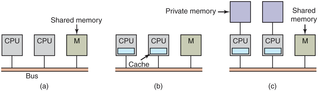
Three bus-based multiprocessors. (a) Without caching. (b) With caching. (c) With caching and private memories.
If the bus is busy when a CPU wants to read or write memory, the CPU just waits until the bus becomes idle. Herein lies the problem with this design. With two or three CPUs, contention for the bus will be manageable; with 32 or 64 it will be unbearable. The system will be totally limited by the bandwidth of the bus, and most of the CPUs will be idle most of the time.
The solution to this problem is to add a cache to each CPU, as depicted in Fig. 8-2(b). The cache can be inside the CPU chip, next to the CPU chip, on the processor board, or some combination of all three. Since many reads can now be satisfied out of the local cache, there will be much less bus traffic, and the system can support more CPUs. In general, caching is not done on an individual word basis but on the basis of 32- or 64-byte blocks. When a word is referenced, its entire block, called a cache line, is fetched into the cache of the CPU touching it.
Each cache block is marked as being either read only (in which case it can be present in multiple caches at the same time) or read-write (in which case it may not be present in any other caches). If a CPU attempts to write a word that is in one or more remote caches, the bus hardware detects the write and puts a signal on the bus informing all other caches of the write. If other caches have a ‘‘clean’’ copy, that is, an exact copy of what is in memory, they can just discard their copies and let the writer fetch the cache block from memory before modifying it. If some other cache has a ‘‘dirty’’ (i.e., modified) copy, it must either write it back to memory before the write can proceed or transfer it directly to the writer over the bus. This set of rules is called a cache-coherence protocol and is one of many.
Yet another possibility is the design of Fig. 8-2(c), in which each CPU has not only a cache, but also a local, private memory which it accesses over a dedicated (private) bus. To use this configuration optimally, the compiler should place all the program text, strings, constants, and other read-only data, stacks, and local variables in the private memories. The shared memory is then used only for writable shared variables. In most cases, this careful placement will reduce bus traffic, but it does require active cooperation from the compiler. It can be done, for example, by allocating part of the address space to the shared memory, the rest to each CPU’s private memory, and putting variables and data structures in the right part.
UMA Multiprocessors Using Crossbar Switches
Even with the best caching, the use of a single bus limits the size of a UMA multiprocessor to about 16 or 32 CPUs. To go beyond that, a different kind of interconnection network is needed. The simplest circuit for connecting n CPUs to k memories is the crossbar switch, shown in Fig. 8-3. Crossbar switches have been used for decades in telephone switching exchanges to connect a group of incoming lines to a set of outgoing lines in an arbitrary way.
Figure 8-3
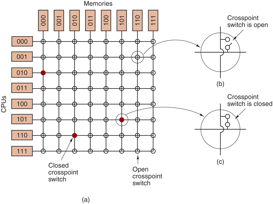
(a) An crossbar switch. (b) An open crosspoint. (c) A closed crosspoint.
At each intersection of a horizontal (incoming) and vertical (outgoing) line is a crosspoint. A crosspoint is a small electronic switch that can be electrically opened or closed, depending on whether the horizontal and vertical lines are to be connected or not. In Fig. 8-3(a), we see three crosspoints closed simultaneously, allowing connections between the (CPU, memory) pairs (010, 000), (101, 101), and (110, 010) at the same time. Many other combinations are also possible. In fact, the number of combinations is equal to the number of different ways eight rooks can be safely placed on a chess board.
One of the nicest properties of the crossbar switch is that it is a nonblocking network, meaning that no CPU is ever denied the connection it needs because some crosspoint or line is already occupied (assuming the memory module itself is available). Not all interconnects have this fine property. Furthermore, no advance planning is needed. Even if seven arbitrary connections are already set up, it is always possible to connect the remaining CPU to the remaining memory.
Contention for memory is still possible, of course, if two CPUs want to access the same module at the same time. Nevertheless, by partitioning the memory into n units, contention is reduced by a factor of n compared to the model of Fig. 8-2.
One of the worst properties of the crossbar switch is the fact that the number of crosspoints grows as With 1000 CPUs and 1000 memory modules, we need a million crosspoints. Such a large crossbar switch is not feasible. Nevertheless, for medium-sized systems, a crossbar design is workable.
UMA Multiprocessors Using Multistage Switching Networks
A completely different multiprocessor design is based on the humble switch shown in Fig. 8-4(a). This switch has two inputs and two outputs. Messages arriving on either input line can be switched to either output line. For our purposes, messages will contain up to four parts, as shown in Fig. 8-4(b). The Module field tells which memory to use. The Address specifies an address within a module. The Opcode gives the operation, such as READ or WRITE. Finally, the optional Value field may contain an operand, such as a 32-bit word to be written on a WRITE. The switch inspects the Module field and uses it to determine if the message should be sent on X or on Y.
Figure 8-4
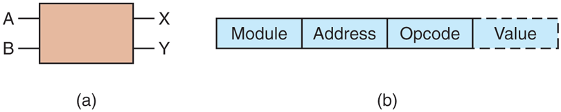
(a) A switch with two input lines, A and B, and two output lines, X and Y. (b) A message format.
Our switches can be arranged in many ways to build larger multistage switching networks (Adams et al., 1987; Garofalakis and Stergiou, 2013; and Kumar and Reddy, 1987). One possibility is the no-frills, cattle-class omega network, illustrated in Fig. 8-5. Here, we have connected eight CPUs to eight memories using 12 switches. More generally, for n CPUs and n memories we would need stages, with switches per stage, for a total of switches, which is a lot better than crosspoints, especially for large values of n.
Figure 8-5
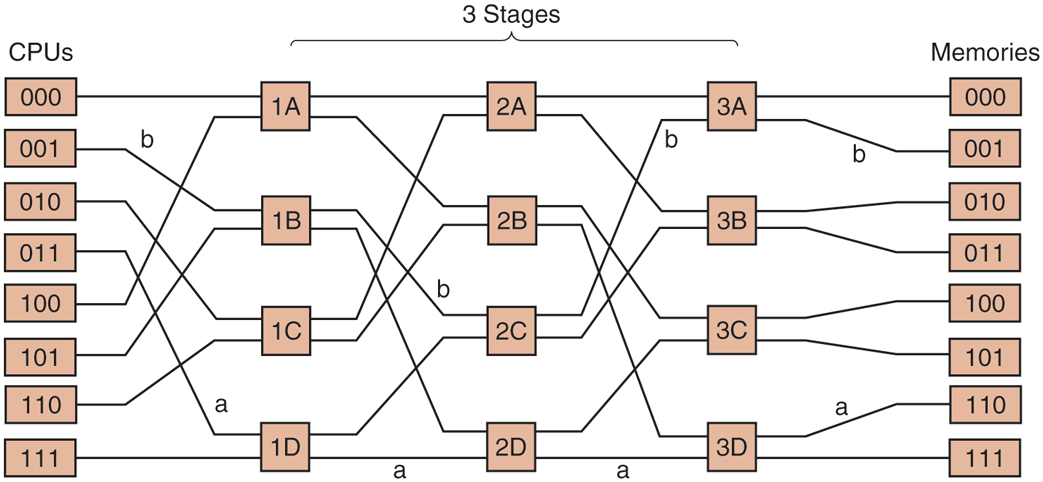
An omega switching network.
The wiring pattern of the omega network is often called the perfect shuffle, since the mixing of the signals at each stage resembles a deck of cards being cut in half and then mixed card-for-card. To see how the omega network works, suppose that CPU 011 wants to read a word from memory module 110. The CPU sends a READ message to switch 1D containing the value 110 in the Module field. The switch takes the first (i.e., leftmost) bit of 110 and uses it for routing. A 0 routes to the upper output and a 1 routes to the lower one. Since this bit is a 1, the message is routed via the lower output to 2D.
All the second-stage switches, including 2D, use the second bit for routing. This, too, is a 1, so the message is now forwarded via the lower output to 3D. Here, the third bit is tested and found to be a 0. Consequently, the message goes out on the upper output and arrives at memory 110, as desired. The path followed by this message is marked in Fig. 8-5 by the letter a.
As the message moves through the switching network, the bits at the left-hand end of the module number are no longer needed. They can be put to good use by recording the incoming line number there, so the reply can find its way back. For path a, the incoming lines are 0 (upper input to 1D), 1 (lower input to 2D), and 1 (lower input to 3D), respectively. The reply is routed back using 011, only reading it from right to left this time.
At the same time all this is going on, CPU 001 wants to write a word to memory module 001. An analogous process happens here, with the message routed via the upper, upper, and lower outputs, respectively, marked by the letter b. When it arrives, its Module field reads 001, representing the path it took. Since these two requests do not use any of the same switches, lines, or memory modules, they can proceed in parallel.
Now consider what would happen if CPU 000 simultaneously wanted to access memory module 000. Its request would come into conflict with CPU 001’s request at switch 3A. One of them would then have to wait. Unlike the crossbar switch, the omega network is a blocking network. Not every set of requests can be processed simultaneously. Conflicts can occur over the use of a wire or a switch, as well as between requests to memory and replies from memory.
Since it is highly desirable to spread the memory references uniformly across the modules, one common technique is to use the low-order bits as the module number. Consider, for example, a byte-oriented address space for a computer that mostly accesses full 32-bit words. The 2 low-order bits will usually be 00, but the next 3 bits will be uniformly distributed. By using these 3 bits as the module number, consecutively words will be in consecutive modules. A memory system in which consecutive words are in different modules is said to be interleaved. Interleaved memories maximize parallelism because most memory references are to consecutive addresses. It is also possible to design switching networks that are nonblocking and offer multiple paths from each CPU to each memory module to spread the traffic better.
NUMA Multiprocessors
Single-bus UMA multiprocessors are generally limited to no more than a few dozen CPUs, and crossbar or switched multiprocessors need a lot of (expensive) hardware and are not that much bigger. To get to more than 100 CPUs, something has to give. Usually, what gives is the idea that all memory modules have the same access time. This concession leads to the idea of NUMA multiprocessors, as mentioned above. Like their UMA cousins, they provide a single address space across all the CPUs, but unlike the UMA machines, access to local memory modules is faster than access to remote ones. Thus all UMA programs will run without change on NUMA machines, but the performance will be worse than on a UMA machine.
NUMA machines have three key characteristics that all of them possess and that together distinguish them from other multiprocessors:
There is a single address space visible to all CPUs.
Access to remote memory is via
LOADandSTOREinstructions.Access to remote memory is slower than access to local memory.
When the access time to remote memory is not hidden (because there is no caching), the system is called NC-NUMA (Non Cache-coherent NUMA). When the caches are coherent, the system is called CC-NUMA (Cache-Coherent NUMA).
A popular approach for building large CC-NUMA multiprocessors is the directory-based multiprocessor. The idea is to maintain a database telling where each cache line is and what its status is. When a cache line is referenced, the database is queried to find out where it is and whether it is clean or dirty. Since this database is queried on every instruction that touches memory, it must be kept in extremely fast special-purpose hardware that can respond in a fraction of a bus cycle.
To make the idea of a directory-based multiprocessor somewhat more concrete, let us consider as a simple (hypothetical) example, a 256-node system, each node consisting of one CPU and 16 MB of RAM connected to the CPU via a local bus. The total memory is bytes and it is divided up into cache lines of 64 bytes each. The memory is statically allocated among the nodes, with 0–16M in node 0, 16M–32M in node 1, etc. The nodes are connected by an interconnection network, as shown in Fig. 8-6(a). Each node also holds the directory entries for the 64-byte cache lines comprising its -byte memory. For the moment, we will assume that a line can be held in at most one cache.
Figure 8-6
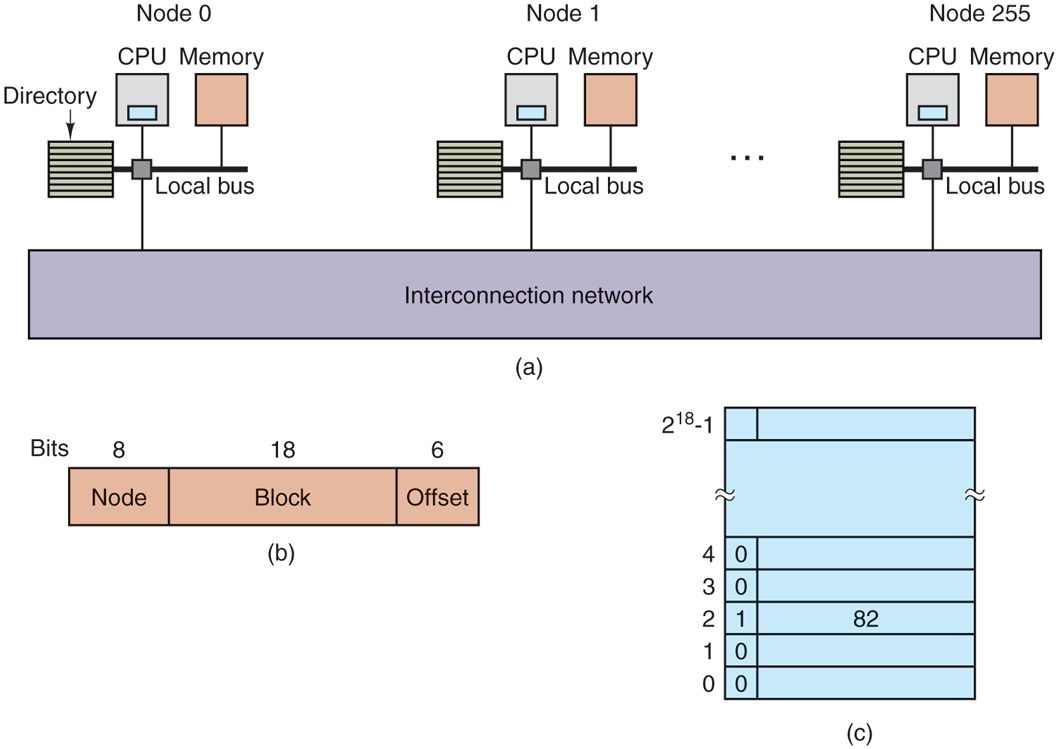
(a) A 256-node directory-based multiprocessor. (b) Division of a 32-bit memory address into fields. (c) The directory at node 36.
To see how the directory works, let us trace a LOAD instruction from CPU 20 that references a cached line. First the CPU issuing the instruction presents it to its MMU, which translates it to a physical address, say, 0x24000108. The MMU splits this address into the three parts shown in Fig. 8-6(b). In decimal, the three parts are node 36, line 4, and offset 8. The MMU sees that the memory word referenced is from node 36, not node 20, so it sends a request message through the interconnection network to the line’s home node, 36, asking whether its line 4 is cached, and if so, where.
When the request arrives at node 36 over the interconnection network, it is routed to the directory hardware. The hardware indexes into its table of entries, one for each of its cache lines, and extracts entry 4. From Fig. 8-6(c), we see that the line is not cached, so the hardware issues a fetch for line 4 from the local RAM and after it arrives sends it back to node 20. It then updates directory entry 4 to indicate that the line is now cached at node 20.
Now let us consider a second request, this time asking about node 36’s line 2. From Fig. 8-6(c) we see that this line is cached at node 82. At this point, the hardware could update directory entry 2 to say that the line is now at node 20 and then send a message to node 82 instructing it to pass the line to node 20 and invalidate its cache. Note that even a so-called ‘‘shared-memory multiprocessor’’ has a lot of message passing going on under the hood.
As a quick aside, let us calculate how much memory is being taken up by the directories. Each node has 16 MB of RAM and 9-bit entries to keep track of that RAM. Thus, the directory overhead is about bits divided by 16 MB or about 1.76%, which is generally acceptable (although it has to be high-speed memory, which increases its cost, of course). Even with 32-byte cache lines the overhead would only be 4%. With 128-byte cache lines, it would be under 1%.
An obvious limitation of this design is that a line can be cached at only one node. To allow lines to be cached at multiple nodes, we would need some way of locating all of them, for example, to invalidate or update them on a write. On many multicore processors, a directory entry therefore consists of a bit vector with one bit per core. A ‘‘1’’ indicates that the cache line is present on the core, and a ‘‘0’’ that it is not. Moreover, each directory entry typically contains a few more bits. As a result, the memory cost of the directory increases considerably. The design of 64-bit systems is more complicated, but the fundamental principles are similar.
Multicore Chips
As chip manufacturing technology improves, transistors are getting smaller and smaller and it is possible to put more and more of them on a chip. This empirical observation is often called Moore’s Law, after Intel co-founder Gordon Moore, who first noticed it. In 1974, the Intel 8080 contained a little over 2000 transistors, while Xeon Nehalem-EX CPUs have over 2 billion transistors.
An obvious question is: ‘‘What do you do with all those transistors?’’ As we discussed in Sec. 1.3.1, one option is to add megabytes of cache to the chip. This option is serious, and chips with 4–32 MB of on-chip cache are common. But at some point increasing the cache size may run the hit rate up only from 99% to 99.5%, which does not improve application performance much.
The other option is to put two or more complete CPUs, usually called cores, on the same chip (technically, on the same die). Chips with 4–64 cores are already common; and you can even buy chips with hundreds of cores. No doubt more cores are on their way. Caches are still crucial and are now spread across the chip. For instance, AMD’s EPYC Milan CPU has up to 64 cores with 2 hardware threads each, giving 128 virtual cores.
In many systems, each core typically has access to multiple levels of cache, from a close-by, small, fast L1 (Level 1) cache to a more distant, bigger, and slower L3 cache, with the L2 in between. Each of the EPYC Milan’s 64 cores has 32 KB of L1 instruction cache and 32 KB of data cache in addition to 512 KB of L2 cache. Finally, the cores share 256 MB of on-board L3 cache.
While the CPUs may or may not share caches (see Fig. 1-8), they always share main memory, and this memory is consistent in the sense that there is always a unique value for each memory word. Special hardware circuitry makes sure that if a word is present in two or more caches and one of the CPUs modifies the word, it is automatically and atomically removed from all the caches in order to maintain consistency. This process is known as snooping.
The result of this design is that multicore chips are just very small multiprocessors. In fact, multicore chips are sometimes called CMPs (Chip MultiProcessors). From a software perspective, CMPs are not really that different from busbased multiprocessors or multiprocessors that use switching networks. However, there are some differences. To start with, on a bus-based multiprocessor, each of the CPUs has its own cache, as in Fig. 8-2(b) and also as in the design of Fig. 1-8(b). The shared-cache design of Fig. 1-8(a) does not occur in other multiprocessors. Nowadays the L3 cache is typically shared. This does not necessarily mean that they are centralized. Often a large, shared cache is partitioned in percore slices. For instance, on a CPU with 8 cores and a 32 MB shared cache, each core has a slice of 4 MB. The slices are shared so that any core can access any slice, but the performance varies. Accessing your local slice is much faster. In other words, we have a NUMA cache.
NUMA issues aside, a shared L2 or L3 cache can affect performance either positively or negatively. If one core needs a lot of cache memory and the others do not, this design allows the cache hog to take whatever it needs. On the other hand, the shared cache also makes it possible for a greedy core to hurt the other cores.
An area in which CMPs differ from their larger cousins is fault tolerance. Because the CPUs are closely connected, failures in shared components may bring down multiple CPUs at once, something unlikely in traditional multiprocessors.
In addition to symmetric multicore chips, where all the cores are identical, another common category of multicore chip is the SoC (System On a Chip). These chips have one or more main CPUs, but also special-purpose cores, such as video and audio decoders, cryptoprocessors, network interfaces, and more, leading to a complete computer system on a chip. The M1 chip, used on some Apple computers and mobile devices, is an SoC with four high-performance, power-hungry cores and four lower-performance, energy-efficient cores. This gives the operating system the ability to run threads on fast cores when that is needed but save energy when it is not.
Manycore Chips
Multicore simply means ‘‘more than one core,’’ but when the number of cores grows well beyond the reach of finger counting, we use another name. Manycore chips are multicores that contain many tens, hundreds, or even thousands of cores. While there is no hard threshold beyond which a multicore becomes a manycore, an easy distinction is that you probably have a manycore if you no longer care about losing one or two cores.
Dual-processor versions of AMD’s EPYC Milan CPU already offer 128 cores in a single chip. Other vendors have also crossed the 100-core barrier with hundreds of cores. A thousand general-purpose cores may be on their way. It is not easy to imagine what to do with a thousand cores, much less how to program them outside of niche applications. For example, a video-editing application working on a 60 frames/sec 2-hour movie might have to apply a complex Photoshop filter to all 432,000 frames. Doing this in parallel on 1024 cores might make the rendering process go much faster.
Another problem with really large numbers of cores is that the machinery needed to keep their caches coherent becomes very complicated and very expensive. Many engineers worry that cache coherence may not scale to many hundreds of cores. Some even advocate that we should give it up altogether. They fear that the cost of coherence protocols in hardware will be so high that all those shiny new cores will not help performance much because the processor is too busy keeping the caches in a consistent state. Worse, it would need to spend way too much memory on the (fast) directory to do so. This is known as the coherency wall.
Consider, for instance, our directory-based cache-coherency solution discussed above. If each directory entry contains a bit vector to indicate which cores contain a particular cache line, the directory entry for a CPU with 1024 cores will be at least 128 bytes long. Since cache lines themselves are rarely larger than 128 bytes, this leads to the awkward situation that the directory entry is larger than the cacheline it tracks. Probably not what we want.
Some engineers argue that the only programming model that has proven to scale to very large numbers of processors is that which employs message passing and distributed memory—and that is what we should expect in future manycore chips also. On the other hand, other processors still provide consistency even at large core counts. Hybrid models are also possible. For instance, a 1024-core chip may be partitioned in 64 islands with 16 cache-coherent cores each, while abandoning cache coherence between the islands.
Thousands of cores are not even that special any more. The most common manycores today, graphics processing units, are found in just about any computer system that is not embedded and has a monitor. A GPU is a processor with dedicated memory and, literally, thousands of itty-bitty cores. Compared to general-purpose processors, GPUs spend more of their transistor budget on the circuits that perform calculations and less on caches and control logic. They are very good for many small computations done in parallel, like rendering polygons in graphics applications. They are not so good at serial tasks. They are also very difficult to program and debug. While GPUs can be useful for operating systems (e.g., encryption or processing of network traffic), it is not likely that much of the operating system itself will run on the GPUs.
Other computing tasks are increasingly handled by the GPU (or similar processors), especially computationally demanding ones that are common in scientific computing. The term used for general-purpose processing on GPUs is (surprise): GPGPU. Unfortunately, programming GPUs efficiently is extremely difficult and requires special programming languages such as OpenGL, or NVIDIA’s proprietary CUDA. An important difference between programming GPUs and programming general-purpose processors is that GPUs are essentially ‘‘single instruction multiple data’’ machines, which means that a large number of cores execute exactly the same instruction but on different pieces of data. This model is great for data parallelism, but poor for task parallelism.
GPUs proved useful for many applications, not just scientific computing or games. For instance, machine learning grew to be an important application. In fact, it grew to be so important that Google started developing a special-purpose processor, known as the TPU (Tensor Processing Unit) although some people prefer the more generic NPU (Neural Processing Unit). It derives from the TensorFlow software that drives many of the machine learning solutions. TPUs combine many simple processing units in such a way as to perform matrix multiplications very efficiently—operations that are common in machine learning. As their impact on operating systems is limited, we will not discuss them further. In the same vein, we do not discuss Network Processing Units (brilliantly abbreviated to NPU also) or the raft of other types application-specific coprocesors around today.
Heterogeneous Multicores
Some chips integrate a GPU, a TPU, and a number of general-purpose cores on the same die. Similarly, SoCs may contain different types of general-purpose core. Systems that integrate multiple different breeds of processors in a single chip are collectively known as heterogeneous multicore processors.
Some of these systems are very heterogeneous in the sense that the different cores have different instruction sets. For instance, this is true for SoCs that have a GPU and/or TPU in addition to general-purpose cores. However, it is also possible to introduce heterogeneity while maintaining the same instruction set. For instance, a CPU can have a small number of ‘‘big’’ cores, with deep pipelines and possibly high clock speeds, and a larger number of ‘‘little’’ cores that are simpler, less powerful, and perhaps run at lower frequencies. The powerful cores are needed for running code that requires fast sequential processing while the little cores are useful for power-efficiency and for tasks that can be executed efficiently in parallel. Examples include ARM’s big.LITTLE and Intel’s Alder Lake architectures.
Programming with Multiple Cores
As has often happened in the past, the hardware is way ahead of the software. While multicore chips are here now, our ability to write applications for them is not. Current programming languages are poorly suited for writing highly parallel programs, and good compilers and debugging tools are scarce on the ground. Few programmers are experts in parallel programming and most know little about dividing work into multiple packages that can run in parallel. Synchronization, eliminating race conditions, and deadlock avoidance are such stuff as really bad dreams are made of, but unfortunately performance suffers horribly if they are not handled well. Semaphores are not the answer.
Beyond these startup problems, it is far from obvious what kind of application really needs hundreds, let alone thousands, of general-purpose cores—especially in home environments. In large server farms, on the other hand, there is often plenty of work for large numbers of cores. For instance, a popular server may easily use a different core for each client request. Similarly, the cloud providers discussed in the previous chapter can soak up the cores to provide a large number of virtual machines to rent out to clients looking for on-demand computing power.
Simultaneous Multithreading
Not only do CPUs have many cores, those cores can support SMT (Simultaneous Multithreading). SMT means that a core offers multiple hardware contexts that are sometimes referred to as hyper-threads. As usual, the hardware folks did not miss their chance to sow confusion in their naming of things, and we emphasize that a hyper-thread is different from the threads we discussed in earlier chapters—it refers to the capability of the hardware to run multiple things, processes or threads, simultaneously on the same core. In other words, each hyper-thread can run a process or a thread (or even a process with multiple user-level threads). For this reason, some people talk about virtual cores instead of hyper-threads.
Indeed, each hyper-thread serves as a virtual core. For instance, it has its own set of registers to run a separate process independently of what is running on the other hyper-thread(s). However, it is not an independent physical core, as resources such as the L1 and L2 caches, the TLB, the execution units, and many other elements are typically shared between the hyper-threads. Incidentally, this also means that the execution of one hyper-thread can easily interfere with that of another thread: if an execution engine is in use by one thread, other threads that want to use it will have to wait. And when one process accesses a new page of virtual memory, the access may remove a TLB entry from the process in the other hyper-thread.
The benefit of hyper-threading is that you get ‘‘almost an extra core’’ for a fraction of the price. The performance benefits of hyper-threads vary. Some workloads can be sped by as much as 30% or more, but for many applications, the difference is much smaller.
8.1.2 Multiprocessor Operating System Types
Let us now turn from multiprocessor hardware to multiprocessor software, in particular, multiprocessor operating systems. Various approaches are possible. Below we will study three of them. Note that all of these are equally applicable to multicore systems as well as systems with discrete CPUs.
Each CPU Has Its Own Operating System
The simplest possible way to organize a multiprocessor operating system is to statically divide memory into as many partitions as there are CPUs and give each CPU its own private memory and its own private copy of the operating system. In effect, the n CPUs then operate as n independent computers. One obvious optimization is to allow all the CPUs to share the operating system code and make private copies of only the operating system data structures, as shown in Fig. 8-7.
Figure 8-7
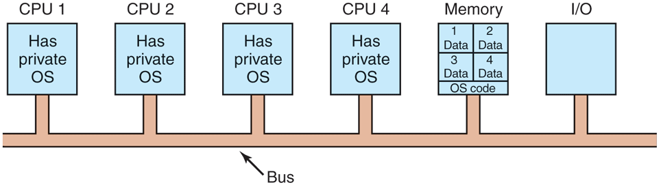
Partitioning multiprocessor memory among four CPUs, but sharing a single copy of the operating system code. The boxes marked Data are the operating system’s private data for each CPU.
This scheme is still better than having n separate computers since it allows all the machines to share a set of disks and other I/O devices, and it also allows the memory to be shared flexibly. For example, even with static memory allocation, one CPU can be given an extra-large portion of the memory so it can handle large programs efficiently. In addition, processes can efficiently communicate with one another by allowing a producer to write data directly into memory and allowing a consumer to fetch it from the place the producer wrote it. Still, from an operating systems’ perspective, having each CPU have its own operating system is as primitive as it gets.
It is worth mentioning four aspects of this design that may not be obvious. First, when a process makes a system call, the system call is caught and handled on its own CPU using the data structures in that operating system’s tables.
Second, since each operating system has its own tables, it also has its own set of processes that it schedules by itself. There is no sharing of processes. If a user logs into CPU 1, all of his processes run on CPU 1. As a consequence, it can happen that CPU 1 is idle while CPU 2 is loaded with work.
Third, there is no sharing of physical pages. It can happen that CPU 1 has pages to spare while CPU 2 is paging continuously. There is no way for CPU 2 to borrow some pages from CPU 1 since the memory allocation is fixed.
Fourth, and worst, if the operating system maintains a buffer cache of recently used disk blocks, each operating system does this independently of the other ones. Thus it can happen that a certain disk block is present and dirty in multiple buffer caches at the same time, leading to inconsistent results. The only way to avoid this problem is to eliminate the buffer caches. Doing so is not hard, but it hurts performance considerably so operating systems always have a buffer cache.
For these reasons, this model is rarely used in production systems any more, although it was used in the early days of multiprocessors, when the goal was to port existing operating systems to some new multiprocessor as fast as possible. In research, the model is making a comeback, but with all sorts of twists. There is something to be said for keeping the operating systems completely separate. If all of the state for each processor is kept local to that processor, there is little to no sharing to lead to consistency or locking problems. Conversely, if multiple processors have to access and modify the same process table, the locking becomes complicated quickly (and crucial for performance). We will say more about this when we discuss the symmetric multiprocessor model below.
Leader-Follower Multiprocessors
A second model is shown in Fig. 8-8. Here, one copy of the operating system and its tables is present on CPU 1 and not on any of the others. All system calls are redirected to CPU 1 for processing there. CPU 1 may also run user processes if there is CPU time left over. This model is called leader-follower since CPU 1 is the leader and all the others are subordinate followers.
Figure 8-8
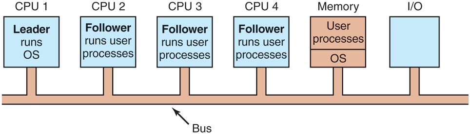
A leader-follower multiprocessor model.
The leader-follower model solves most of the problems of the first model. There is a single data structure (e.g., one list or a set of prioritized lists) that keeps track of ready processes. When a CPU goes idle, it asks the operating system on CPU 1 for a process to run and is assigned one. Thus, it can never happen that one CPU is idle while another is overloaded. Similarly, pages can be allocated among all the processes dynamically and there is only one buffer cache, so inconsistencies never occur.
The problem with this model is that with many CPUs, the leader will become a bottleneck. After all, it must handle all system calls from all CPUs. If, say, 10% of all time is spent handling system calls, then 10 CPUs will pretty much saturate the leader, and with 20 CPUs it will be completely overloaded. Thus this model is simple and workable for small multiprocessors, but for large ones it fails.
Symmetric Multiprocessors
Our third model, the SMP (Symmetric MultiProcessor), eliminates this asymmetry. There is one copy of the operating system in memory, but any CPU can run it. When a system call is made, the CPU on which the system call was made traps to the kernel and processes the system call. The SMP model is illustrated in Fig. 8-9.
Figure 8-9
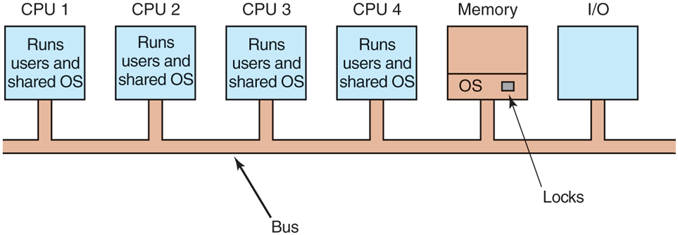
The SMP multiprocessor model.
This model balances processes and memory dynamically, since there is only one set of operating system tables. It also eliminates the leader CPU bottleneck, since there is no leader, but it introduces its own problems. In particular, if two or more CPUs are running operating system code at the same time, disaster may well result. Imagine two CPUs simultaneously picking the same process to run or claiming the same free memory page. The simplest way around these problems is to associate a mutex (i.e., lock) with the operating system, making the whole system one big critical region. When a CPU wants to run operating system code, it must first acquire the mutex. If the mutex is locked, it just waits. In this way, any CPU can run the operating system, but only one at a time. This approach is sometimes called a big kernel lock.
This model works, but is almost as bad as the leader-follower model. Again, suppose that 10% of all run time is spent inside the operating system. With 20 CPUs, there will be long queues of CPUs waiting to get in. Fortunately, it is easy to improve. Many parts of the operating system are independent of one another. For example, there is no problem with one CPU running the scheduler while another CPU is handling a file-system call and a third one is processing a page fault.
This observation leads to splitting the operating system up into multiple independent critical regions that do not interact with one another. Each critical region is protected by its own mutex, so only one CPU at a time can execute it. In this way, far more parallelism can be achieved. However, it may well happen that some tables, such as the process table, are used by multiple critical regions. For example, the process table is needed for scheduling, but also for the fork system call and also for signal handling. Each table that may be used by multiple critical regions needs its own mutex. In this way, each critical region can be executed by only one CPU at a time and each critical table can be accessed by only one CPU at a time.
Most modern multiprocessors use this arrangement. The hard part about writing the operating system for such a machine is not that the actual code is so different from a regular operating system. It is not. The hard part is splitting it into critical regions that can be executed concurrently by different CPUs without interfering with one another, not even in subtle, indirect ways. In addition, every table used by two or more critical regions must be separately protected by a mutex and all code using the table must use the mutex correctly.
Furthermore, great care must be taken to avoid deadlocks. If two critical regions both need table A and table B, and one of them claims A first and the other claims B first, sooner or later a deadlock will occur and nobody will know why. In theory, all the tables could be assigned integer values and all the critical regions could be required to acquire tables in increasing order. This strategy avoids deadlocks, but it requires the programmer to think very carefully about which tables each critical region needs and to make the requests in the right order.
As the code evolves over time, a critical region may need a new table it did not previously need. If the programmer is new and does not understand the full logic of the system, then the temptation will be to just grab the mutex on the table at the point it is needed and release it when it is no longer needed. However reasonable this may appear, it may lead to deadlocks, which the user will perceive as the system freezing. Getting it right is not easy and keeping it right over a period of years in the face of changing programmers is very difficult, so the whole approach is very error-prone.
8.1.3 Multiprocessor Synchronization
The CPUs in a multiprocessor frequently need to synchronize. We just saw the case in which kernel critical regions and tables have to be protected by mutexes. Let us now take a close look at how this synchronization actually works in a multiprocessor. It is far from trivial, as we will soon see.
To start with, proper synchronization primitives are really needed. If a process on a uniprocessor machine (just one CPU) makes a system call that requires accessing some critical kernel table, the kernel code can just disable interrupts before touching the table. It can then do its work knowing that it will be able to finish without any other process sneaking in and touching the table before it is finished. On a multiprocessor, disabling interrupts affects only the CPU doing the disable. Other CPUs continue to run and can still touch the critical table. As a consequence, a proper mutex protocol must be used and respected by all CPUs to guarantee that mutual exclusion works.
The heart of any practical mutex protocol is a special instruction that allows a memory word to be inspected and set in one indivisible operation. We saw how TSL (Test and Set Lock) was used in Fig. 2-25 to implement critical regions. As we discussed earlier, what this instruction does is read out a memory word and store it in a register. Simultaneously, it writes a 1 (or some other nonzero value) into the memory word. Of course, it takes two bus cycles to perform the memory read and memory write. On a uniprocessor, as long as the instruction cannot be broken off halfway, TSL always works as expected.
Now think about what could happen on a multiprocessor. In Fig. 8-10, we see the worst-case timing, in which memory word 1000, being used as a lock, is initially 0. In step 1, CPU 1 reads out the word and gets a 0. In step 2, before CPU 1 has a chance to rewrite the word to 1, CPU 2 gets in and also reads the word out as a 0. In step 3, CPU 1 writes a 1 into the word. In step 4, CPU 2 also writes a 1 into the word. Both CPUs got a 0 back from the TSL instruction, so both of them now have access to the critical region and the mutual exclusion fails.
Figure 8-10
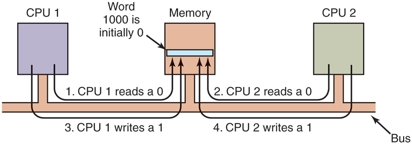
The TSL instruction can fail if the bus cannot be locked. These four steps show a sequence of events where the failure is demonstrated.
To prevent this problem, the TSL instruction must first lock the bus, preventing other CPUs from accessing it, then do both memory accesses, then unlock the bus. Typically, locking the bus is done by requesting the bus using the usual bus request protocol, then asserting (i.e., setting to a logical 1 value) some special bus line until both cycles have been completed. As long as this special line is being asserted, no other CPU will be granted bus access. This instruction can only be implemented on a bus that has the necessary lines and (hardware) protocol for using them. Modern buses all have these facilities, but on earlier ones that did not, it was not possible to implement TSL correctly. This is why Peterson’s protocol was invented: to synchronize entirely in software (Peterson, 1981).
If TSL is correctly implemented and used, it guarantees that mutual exclusion can be made to work. However, this mutual exclusion method uses a spin lock because the requesting CPU just sits in a tight loop testing the lock as fast as it can. Not only does it completely waste the time of the requesting CPU (or CPUs), but it may also put a massive load on the bus or memory, seriously slowing down all other CPUs trying to do their normal work.
At first glance, it might appear that the presence of caching should eliminate the problem of bus contention, but it does not. In theory, once the requesting CPU has read the lock word, it should get a copy in its cache. As long as no other CPU attempts to use the lock, the requesting CPU should be able to run out of its cache. When the CPU owning the lock writes a 0 to it to release it, the cache protocol automatically invalidates all copies of it in remote caches, requiring the correct value to be fetched again.
The problem is that caches operate in blocks of 32 or 64 bytes. Usually, the words surrounding the lock are needed by the CPU holding the lock. Since the TSL instruction is a write (because it modifies the lock), it needs exclusive access to the cache block containing the lock. Therefore, every TSL invalidates the block in the lock holder’s cache and fetches a private, exclusive copy for the requesting CPU. As soon as the lock holder touches a word adjacent to the lock, the cache block is moved to its machine. Consequently, the entire cache block containing the lock is constantly being shuttled between the lock owner and the lock requester, generating even more bus traffic than individual reads on the lock word would have.
If we could get rid of all the TSL-induced writes on the requesting side, we could reduce the cache thrashing appreciably. This goal can be accomplished by having the requesting CPU first do a pure read to see if the lock is free. Only if the lock appears to be free does it do a TSL to actually acquire it. The result of this small change is that most of the polls are now reads instead of writes. If the CPU holding the lock is only reading the variables in the same cache block, they can each have a copy of the cache block in shared read-only mode, eliminating all the cache-block transfers.
When the lock is eventually freed, the owner does a write, which requires exclusive access, thus invalidating all copies in remote caches. On the next read by the requesting CPU, the cache block will be reloaded. Note that if two or more CPUs are contending for the same lock, it can happen that both see that it is free simultaneously, and both do a TSL simultaneously to acquire it. Only one of these will succeed, so there is no race condition here because the real acquisition is done by the TSL instruction, and it is atomic. Seeing that the lock is free and then trying to grab it immediately with a TSL does not guarantee that you get it. Someone else might win, but for the correctness of the algorithm, it does not matter who gets it. Success on the pure read is merely a hint that this would be a good time to try to acquire the lock, but it is not a guarantee that the acquisition will succeed.
Another way to reduce bus traffic is to use the well-known Ethernet binary exponential backoff algorithm (Anderson, 1990). Instead of continuously polling, as in Fig. 2-25, a delay loop can be inserted between polls. Initially the delay is one instruction. If the lock is still busy, the delay is doubled to two instructions, then four instructions, and so on up to some maximum. A low maximum gives a fast response when the lock is released, but wastes more bus cycles on cache thrashing. A high maximum reduces cache thrashing at the expense of not noticing that the lock is free so quickly. Binary exponential backoff can be used with or without the pure reads preceding the TSL instruction.
An even better idea is to give each CPU wishing to acquire the mutex its own private lock variable to test, as illustrated in Fig. 8-11 (Mellor-Crummey and Scott, 1991). The variable should reside in an otherwise unused cache block to avoid conflicts. The algorithm works by having a CPU that fails to acquire the lock allocate a lock variable and attach itself to the end of a list of CPUs waiting for the lock. When the current lock holder exits the critical region, it frees the private lock that the first CPU on the list is testing (in its own cache). This CPU then enters the critical region. When it is done, it frees the lock its successor is using, and so on. Although the protocol is somewhat complicated (to avoid having two CPUs attach themselves to the end of the list simultaneously), it is efficient and starvation free. For all the details, readers should consult the paper.
Figure 8-11
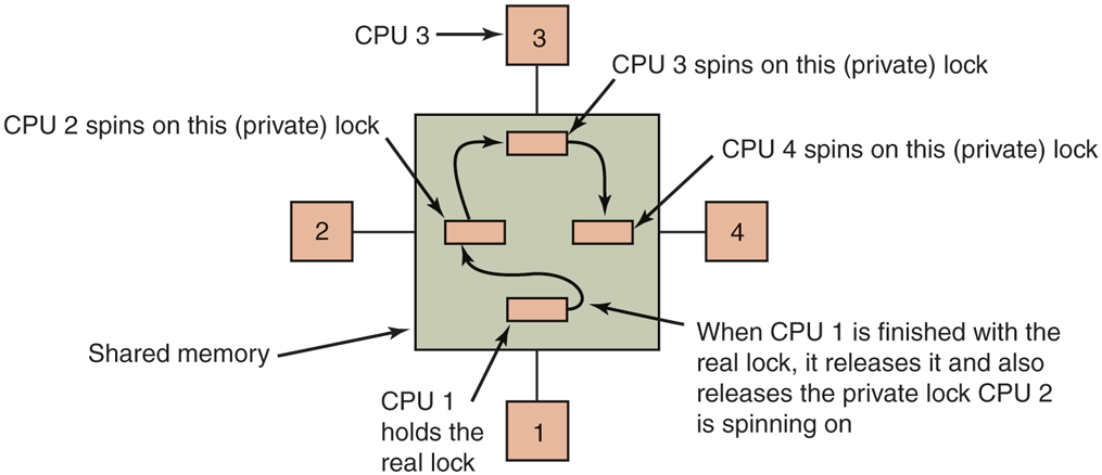
Use of multiple locks to avoid cache thrashing.
Spinning vs. Switching
So far we have assumed that a CPU needing a locked mutex just waits for it, by polling continuously, polling intermittently, or attaching itself to a list of waiting CPUs. Sometimes, there is no alternative for the requesting CPU to just waiting. For example, suppose that some CPU is idle and needs to access the shared ready list to pick a process to run. If the ready list is locked, the CPU cannot just decide to suspend what it is doing and run another process, as doing that would require reading the ready list. It must wait until it can acquire the ready list.
However, in other cases, there is a choice. For example, if some thread on a CPU needs to access the file system buffer cache and it is currently locked, the CPU can decide to switch to a different thread instead of waiting. The issue of whether to spin or to do a thread switch has been a matter of much research, some of which will be discussed below. Note that this issue does not occur on a uniprocessor because spinning does not make much sense when there is no other CPU to release the lock. If a thread tries to acquire a lock and fails, it is always blocked to give the lock owner a chance to run and release the lock.
Assuming that spinning and doing a thread switch are both feasible options, the trade-off is as follows. Spinning wastes CPU cycles directly. Testing a lock repeatedly is not productive work. Switching, however, also wastes CPU cycles, since the current thread’s state must be saved, the lock on the ready list must be acquired, a thread must be selected, its state must be loaded, and it must be started. Furthermore, the CPU cache will contain all the wrong blocks, so many expensive cache misses will occur as the new thread starts running. TLB faults are also likely. Eventually, a switch back to the original thread must take place, with more cache misses following it. The cycles spent doing these two context switches plus all the cache misses are wasted.
If it is known that mutexes are generally held for, say, and it takes 1 msec to switch from the current thread and 1 msec to switch back later, it is more efficient just to spin on the mutex. On the other hand, if the average mutex is held for 10 msec, it is worth the trouble of making the two context switches. The trouble is that critical regions can vary considerably, so which approach is better?
One design is to always spin. A second design is to always switch. But a third design is to make a separate decision each time a locked mutex is encountered. At the time the decision has to be made, it is not known whether it is better to spin or switch, but for any given system, it is possible to make a trace of all activity and analyze it later offline. Then it can be said in retrospect which decision was the best one and how much time was wasted in the best case. This hindsight algorithm then becomes a benchmark against which feasible algorithms can be measured.
This problem has been studied by researchers for decades (Ousterhout, 1982). Most work uses a model in which a thread failing to acquire a mutex spins for some period of time. If this threshold is exceeded, it switches. In some cases, the threshold is fixed, typically the known overhead for switching to another thread and then switching back. In other cases, it is dynamic, depending on the observed history of the mutex being waited on.
The best results are achieved when the system keeps track of the last few observed spin times and assumes that this one will be similar to the previous ones. For example, assuming a 1-msec context switch time again, a thread will spin for a maximum of 2 msec, but observe how long it actually spun. If it fails to acquire a lock and sees that on the previous three runs it waited an average of it should spin for 2 msec before switching. However, if it sees that it spun for the full 2 msec on the previous attempts, it should switch immediately and not spin.
Some modern processors, including the x86, offer special instructions to make the waiting more efficient in terms of reducing power consumption. For instance, the MONITOR/MWAIT instructions on x86 allow a program to block until some other processor modifies the data in a previously defined memory area. Specifically, the MONITOR instruction defines an address range that should be monitored for writes. The MWAIT instruction then blocks the thread until someone writes to the area. Effectively, the thread is spinning, but without burning many cycles needlessly. On notebook computers, this does not drain the battery as much.
8.1.4 Multiprocessor Scheduling
Before looking at how scheduling is done on multiprocessors, it is necessary to determine what is being scheduled. Back in the old days, when all processes were single threaded, processes were scheduled—there was nothing else schedulable. All modern operating systems support multithreaded processes, which makes scheduling more complicated.
It matters whether the threads are kernel threads or user threads. If threading is done by a user-space library and the kernel knows nothing about the threads, then scheduling happens on a per-process basis as it always did. If the kernel does not even know threads exist, it can hardly schedule them.
With kernel threads, the picture is different. Here, the kernel is aware of all the threads and can pick and choose among the threads belonging to a process. In these systems, the trend is for the kernel to pick a thread to run, with the process it belongs to having only a small role (or maybe none) in the thread-selection algorithm. Below we will talk about scheduling threads, but of course, in a system with single-threaded processes or threads implemented in user space, it is the processes that are scheduled.
Process vs. thread is not the only scheduling issue. On a uniprocessor, scheduling is one dimensional. The only question that must be answered (repeatedly) is: ‘‘Which thread should be run next?’’ On a multiprocessor, scheduling has two dimensions. The scheduler has to decide which thread to run and which CPU to run it on. This extra dimension greatly complicates scheduling on multiprocessors.
Another complicating factor is that in some systems all of the threads are unrelated, belonging to different processes and having nothing to do with one another. In others, they come in groups, all belonging to the same application and working together. An example of the former situation is a server system in which independent users start up separate, independent processes. The threads of different processes are unrelated, and each one can be scheduled without regard to the other ones.
An example of the latter situation occurs regularly in program development environments. Large systems often consist of some number of header files containing macros, type definitions, and variable declarations that are used by the actual code files. When a header file is changed, all the code files that include it must be recompiled. The program make is commonly used to manage development. When make is invoked, it starts the compilation of only those code files that must be recompiled on account of changes to the header or code files. Object files that are still valid are not regenerated.
The original version of make did its work sequentially, but newer versions designed for multiprocessors can start up all the compilations at once. If 10 compilations are needed, it does not make sense to schedule 9 of them to run immediately and leave the last one until much later since the user will not perceive the work as completed until the last one has finished. In this case, it makes sense to regard the threads doing the compilations as a single group and to take that into account when scheduling them.
Moreoever, sometimes it is useful to schedule threads that communicate extensively, say in a producer-consumer fashion, not just at the same time, but also close together in space. For instance, they may benefit from sharing caches. Likewise, in NUMA architectures, it may help if they access memory that is close by.
Time Sharing
Let us first address the case of scheduling independent threads; later we will consider how to schedule related threads. The simplest scheduling algorithm for dealing with unrelated threads is to have a single systemwide data structure for ready threads, possibly just a list, but more likely a set of lists for threads at different priorities as depicted in Fig. 8-12(a). Here, the 16 CPUs are all currently busy, and a prioritized set of 14 threads are waiting to run. The first CPU to finish its current work (or have its thread block) is CPU 4, which then locks the scheduling queues and selects the highest-priority thread, A, as shown in Fig. 8-12(b). Next, CPU 12 goes idle and chooses thread B, as illustrated in Fig. 8-12(c). As long as the threads are completely unrelated, doing scheduling this way is a reasonable choice and it is very simple to implement efficiently.
Figure 8-12
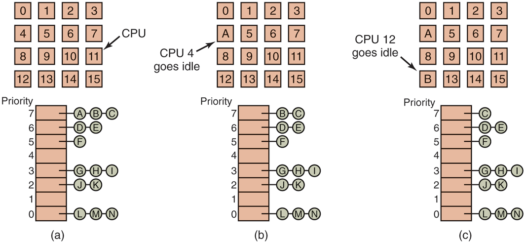
Using a single data structure for scheduling a multiprocessor.
Having a single scheduling data structure used by all CPUs timeshares the CPUs, much as they would be in a uniprocessor system. It also provides automatic load balancing because it can never happen that one CPU is idle while others are overloaded. Two disadvantages of this approach are the potential contention for the scheduling data structure as the number of CPUs grows and the usual overhead in doing a context switch when a thread blocks for I/O.
It is also possible that a context switch happens when a thread’s quantum expires. On a multiprocessor, that has certain properties not present on a uniprocessor. Suppose that the thread happens to hold a spin lock when its quantum expires. Other CPUs waiting on the spin lock just waste their time spinning until that thread is scheduled again and releases the lock. On a uniprocessor, spin locks are rarely used, so if a process is suspended while it holds a mutex, and another thread starts and tries to acquire the mutex, it will be immediately blocked, so little time is wasted.
To get around this anomaly, some systems use smart scheduling, in which a thread acquiring a spin lock sets a processwide flag to show that it currently has a spin lock (Zahorjan et al., 1991). When it releases the lock, it clears the flag. The scheduler then does not stop a thread holding a spin lock, but instead gives it a little more time to complete its critical region and release the lock.
Another issue that plays a role in scheduling is the fact that while all CPUs are equal, some CPUs are more equal. In particular, when thread A has run for a long time on CPU k, CPU k’s cache will be full of A’s blocks. If A gets to run again soon, it may perform better if it is run on CPU k, because k’s cache may still contain some of A’s blocks. Having cache blocks preloaded will increase the cache hit rate and thus the thread’s speed. In addition, the TLB may also contain the right pages, reducing TLB faults.
Some multiprocessors take this effect into account and use what is called affinity scheduling (Vaswani and Zahorjan, 1991). The basic idea here is to make a serious effort to have a thread run on the same CPU it ran on last time. One way to create this affinity is to use a two-level scheduling algorithm. When a thread is created, it is assigned to a CPU, for example, based on which one has the smallest load at that moment. This assignment of threads to CPUs is the top level of the algorithm. As a result, each CPU acquires its own collection of threads.
The actual scheduling of the threads is the bottom level of the algorithm. It is done by each CPU separately, using priorities or some other means. By trying to keep a thread on the same CPU for its entire lifetime, cache affinity is maximized. However, if a CPU has no threads to run, it takes one from another CPU rather than go idle.
Two-level scheduling has three benefits. First, it distributes the load roughly evenly over the available CPUs. Second, advantage is taken of cache affinity where possible. Third, by giving each CPU its own ready list, contention for the ready lists is minimized because attempts to use another CPU’s ready list are relatively infrequent.
Space Sharing
The other general approach to multiprocessor scheduling can be used when threads are related to one another in some way. Earlier we mentioned the example of parallel make as one case. It also often occurs that a single process has multiple threads that work together. For example, if the threads of a process communicate a lot, it is useful to have them running at the same time. Scheduling multiple threads at the same time across multiple CPUs is called space sharing.
The simplest space-sharing algorithm works like this. Assume that an entire group of related threads is created at once. At the time it is created, the scheduler checks to see if there are as many free CPUs as there are threads. If there are, each thread is given its own dedicated (i.e., nonmultiprogrammed) CPU and they all start. If there are not enough CPUs, none of the threads are started until enough CPUs are available. Each thread holds onto its CPU until it terminates, at which time the CPU is put back into the pool of available CPUs. If a thread blocks on I/O, it continues to hold the CPU, which is simply idle until the thread wakes up. When the next batch of threads appears, the same algorithm is applied.
At any instant of time, the set of CPUs is statically partitioned into some number of partitions, each one running the threads of one process. In Fig. 8-13, we have partitions of sizes 4, 6, 8, and 12 CPUs, with 2 CPUs unassigned, for example. As time goes on, the number and size of the partitions will change as new threads are created and old ones finish and terminate.
Figure 8-13
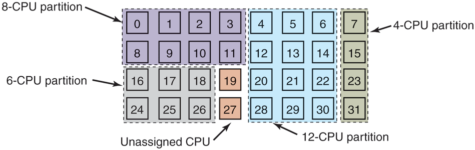
A set of 32 CPUs split into four partitions, with two CPUs available.
Periodically, scheduling decisions have to be made. In uniprocessor systems, shortest job first is a well-known algorithm for batch scheduling. The analogous algorithm for a multiprocessor is to choose the process needing the smallest number of CPU cycles, that is, the thread whose is the smallest of the candidates. However, in practice, this information is rarely available, so the algorithm is hard to carry out. In fact, studies have shown that, in practice, beating first-come, first-served is hard to do (Krueger et al., 1994).
In this simple partitioning model, a thread just asks for some number of CPUs and either gets them all or has to wait until they are available. A different approach is for threads to actively manage the degree of parallelism. One method for managing the parallelism is to have a central server that keeps track of which threads are running and want to run and what their minimum and maximum CPU requirements are (Tucker and Gupta, 1989). Periodically, each application sends a query to the central server to ask how many CPUs it may use. It then adjusts the number of threads up or down to match what is available.
For example, a Web server can have 5, 10, 20, or any other number of threads running in parallel. If it currently has 10 threads and there is suddenly more demand for CPUs and it is told to drop to 5, when the next five threads finish their current work, they are told to exit instead of being given new work. This scheme allows the partition sizes to vary dynamically to match the current workload better than the fixed system of Fig. 8-13.
Gang Scheduling
A clear advantage of space sharing is the elimination of multiprogramming, which eliminates the context-switching overhead. However, an equally clear disadvantage is the time wasted when a CPU blocks and has nothing at all to do until it becomes ready again. Consequently, people have looked for algorithms that attempt to schedule in both time and space together, especially for threads that create multiple threads, which usually need to communicate with one another.
To see the kind of problem that can occur when the threads of a process are independently scheduled, consider a system with threads and belonging to process A and threads and belonging to process B. Threads and are timeshared on CPU 0; threads and are timeshared on CPU 1. Threads and need to communicate often. The communication pattern is that sends a message, with then sending back a reply to followed by another such sequence, common in client-server situations. Suppose luck has it that and start first, as shown in Fig. 8-14.
Figure 8-14
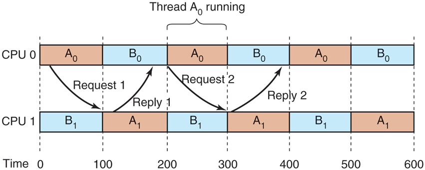
Communication between two threads belonging to thread A that are running out of phase.
In time slice 0, sends a request, but does not get it until it runs in time slice 1 starting at 100 msec. It sends the reply immediately, but does not get the reply until it runs again at 200 msec. The net result is one request-reply sequence every 200 msec. Not very good performance.
The solution to this problem is gang scheduling, which is an outgrowth of coscheduling (Ousterhout, 1982). Gang scheduling has three parts:
Groups of related threads are scheduled as a unit, a gang.
All members of a gang run at once on different timeshared CPUs.
All gang members start and end their time slices together.
The trick that makes gang scheduling work is that all CPUs are scheduled synchronously. Doing this means that time is divided into discrete quanta as we had in Fig. 8-14. At the start of each new quantum, all the CPUs are rescheduled, with a new thread being started on each one. At the start of the next quantum, another scheduling event happens. In between, no scheduling is done. If a thread blocks, its CPU stays idle until the end of the quantum.
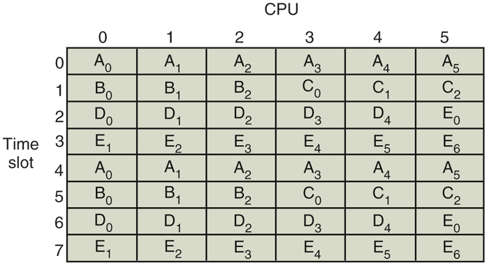
An example of how gang scheduling works is given in Fig. 8-15. Here, we have a multiprocessor with six CPUs being used by five processes, A through E, with a total of 24 ready threads. During time slot 0, threads through are scheduled and run. During time slot 1, threads and are scheduled and run. During time slot 2, D’s five threads and get to run. The remaining six threads belonging to thread E run in time slot 3. Then the cycle repeats, with slot 4 being the same as slot 0, and so on.
Figure 8-15
Gang scheduling.
The idea of gang scheduling is to have all the threads of a process run together, at the same time, on different CPUs, so that if one of them sends a request to another one, it will get the message almost immediately and be able to reply almost immediately. In Fig. 8-15, since all the A threads are running together, during one quantum, they may send and receive a very large number of messages in one quantum, thus eliminating the problem of Fig. 8-14.
Scheduling for Security
As we have seen, security issues complicate just about every operating system activity and scheduling is no exception. Since processes and threads running on the same core in different hardware threads (or hyper-threads) share the core’s resources (such as the cache and the TLB), the activity of one process on the core interferes with that of another. In this section, we briefly explain how an attacker process can learn a secret from a victim process on a core with a shared TLB for code pages. However, this is fairly advanced stuff and we will have more to say about such side channel attacks in Chap. 9.
Suppose we have a core with a fully shared TLB and on one of the core’s hyper-threads we run a program that uses a secret key (which is just a sequence of bits) to encrypt blocks of data provided by the user, for instance in a file, and sends it to a remote server. An attacker on the second hyper-thread wants to know the secret key, but the process is owned by someone else and all she can do is feed the program with data blocks. How will she learn the key?
The trick is to use knowledge about the algorithm. Many cryptographic algorithms encrypt and decrypt data by means of clever mathematical operations that depend on each bit in the key. So, the encryption routine will iterate over the key and for each key bit, it will execute, say, function if the key bit is 0, and function otherwise. In pseudo-code:
for (every bit b in key) {if (b == 0) thenelse}
If and are stored on different pages in memory, say and their execution also reference different pages in the TLB. For an attacker, it would be interesting to learn the sequence of pages used by the other process as it immediately reveals the secret key. Of course, the process will access other pages also, so there is some noise. Even so, suppose she is able to observe the following sequence:
There is a clear pattern. The first pages, and are probably related to start-up code, but after that we see a sequence where the process accesses either or after accessing (where corresponds to the loop instructions).
Although the attacker cannot see the pages that the victim accesses directly, she can use a side channel to observe them indirectly. The trick is to observe her own process’ memory accesses and see whether they are affected by interference from the victim process. To do so, she creates a program with a large number of virtual pages, enough to cover the entire TLB. The program does not take up much physical memory as each code page maps to a single physical page that contains only a few instructions: to measure the number of clock cycles to jump to the next code page. In other words, it obtains the value of the CPU cycle counter, jumps to the virtual address of the next code page, gets the CPU cycle counter again, and calculates the difference. What good does this do? Well, if it took many CPU cycles to jump to the next page, it probably means that there was a TLB miss. That miss was presumably caused by the execution of program code in the victim process. Specifically, every slow jump corresponds to a page accessed by the victim. By observing the sequence of slow pages, the attacker can reconstruct, at least approximately, the sequence of accesses in the victim and from that derive the key.
In practice, side channel attacks can get much more complicated and generally have to deal with less ideal circumstances, for example, due to spurious memory accesses, for instance, by the kernel. However, there are many ways to leak data on a shared core, and many shared resources besides the TLB to do it. Especially after the disclosure of the Meltdown and Spectre vulnerabilities in modern processors in 2018 (Xiong and Szefer, 2021), people got very nervous about running mutually non-trusting programs on the same core.
What does any of this have to do with scheduling, you ask? Since the side channels are particularly problematic for untrusted code that runs on the same core, much work has gone into making sure that processes or threads from different security domains do not run simultaneously on the same core. For instance, the core scheduler on Windows Hyper-V hypervisor guarantees that it will never assign threads from more than one virtual machine to the same physical core. If there is no second from the same virtual machine, it will simply leave the second hyper-thread unused. In fact, it even allows each virtual machine to indicate which threads can run together.
The core scheduler makes it harder for attackers to use specific side channels, but it does not remove all side channels. For instance, in the above example any attack that occurs inside a single virtual machine is still possible. Even so, SMT is problematic from a security perspective and some operating systems, such as OpenBSD, have now disabled it by default—allegedly as a result of the TLB research by one of the authors of this book. (Sorry!)