8 Multiple Processor Systems
Since its inception, the computer industry has been driven by an endless quest for more and more computing power. The ENIAC could perform 300 operations per second, easily 1000 times faster than any calculator before it, yet people were not satisfied with it. We now have machines millions of times faster than the ENIAC, and still there is a demand for yet more horsepower. Astronomers are trying to make sense of the universe, biologists are trying to understand the implications of the human genome, and aeronautical engineers are interested in building safer and more efficient aircraft, and all want more CPU cycles. However much computing power there is, it is never enough.
In the past, the solution was always to make the clock run faster. Unfortunately, we have begun to hit some fundamental limits on clock speed. According to Einstein’s special theory of relativity, no electrical signal can propagate faster than the speed of light, which is about 30 cm/nsec in vacuum and about 20 cm/nsec in copper wire or optical fiber. This means that in a computer with a 10-GHz clock, the signals cannot travel more than 2 cm in total. For a 100-GHz computer, the total path length is at most 2 mm. A 1-THz (1000-GHz) computer will have to be smaller than 100 microns, just to let the signal get from one end to the other and back once within a single clock cycle.
Making computers this small may be possible, but then we hit another fundamental problem: heat dissipation. The faster the computer runs, the more heat it generates, and the smaller the computer, the harder it is to get rid of this heat. Already on high-end x86 systems, the CPU cooler is bigger than the CPU itself. All in all, going from 1 MHz to 1 GHz simply required incrementally better engineering of the chip manufacturing process. Going from 1 GHz to 1 THz is going to require a radically different approach.
One approach to greater speed is through massively parallel computers. These machines consist of many CPUs, each of which runs at ‘‘normal’’ speed (whatever that may mean in a given year), but which collectively have far more computing power than a single CPU. Systems with tens of thousands of CPUs are now commercially available. Systems with 1 million CPUs are already being built in the lab (Plana et al., 2020). While there are other potential approaches to greater speed, such as biological computers, in this chapter we will focus on systems with multiple conventional CPUs.
Highly parallel computers are frequently used for heavy-duty number crunching. Problems such as predicting the weather, modeling airflow around an aircraft wing, simulating the world economy, or understanding drug-receptor interactions in the brain are all computationally intensive. Their solutions require long runs on many CPUs at once. The multiple processor systems discussed in this chapter are widely used for these and similar problems in science and engineering, among other areas.
Another relevant development is the incredibly rapid growth of the Internet. It was originally designed as a prototype for a fault-tolerant military control system, then became popular among academic computer scientists, and long ago acquired many new uses. One of these is linking up thousands of computers all over the world to work together on large scientific problems. In a sense, a system consisting of 1000 computers spread all over the world is no different than one consisting of 1000 computers in a single room, although the delay and other technical characteristics are different. We will also consider these systems in this chapter.
Putting 1 million unrelated computers in a room is easy to do provided that you have enough money and a sufficiently large room. Spreading 1 million unrelated computers around the world is even easier since it finesses the second problem. The trouble comes in when you want them to communicate with one another to work together on a single problem. As a consequence, a great deal of work has been done on interconnection technology, and different interconnect technologies have led to qualitatively different kinds of systems and different software organizations.
All communication between electronic (or optical) components ultimately comes down to sending messages—well-defined bit strings—between them. The differences are in the time scale, distance scale, and logical organization involved. At one extreme are the shared-memory multiprocessors, in which somewhere between 2 and about 1000 CPUs communicate via a shared memory. In this model, every CPU has equal access to the entire physical memory, and can read and write individual words using LOAD and STORE instructions. Accessing a memory word usually takes 1–10 nsec. As we shall see, it is now common to put more than one processing core on a single CPU chip, with the cores sharing access to main memory (and often sharing caches). In other words, the model of shared-memory multicomputers may be implemented using physically separate CPUs, multiple cores on a single CPU, or a combination. While this model, illustrated in Fig. 8-1(a), sounds simple, actually implementing it is not really so simple and usually involves considerable message passing under the covers, as we will explain shortly. However, this message passing is invisible to the programmers.
Figure 8-1
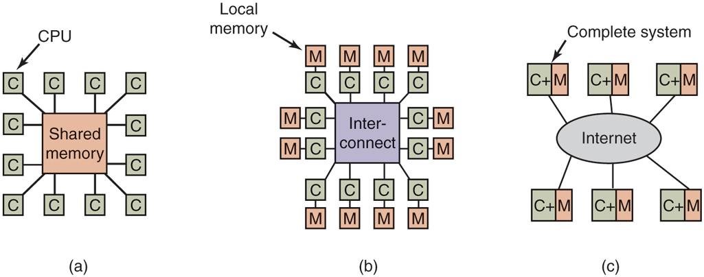
(a) A shared-memory multiprocessor. (b) A message-passing multicomputer. (c) A wide area distributed system.
Next comes the system of Fig. 8-1(b) in which the CPU-memory pairs are connected by a high-speed interconnect. This kind of system is called a message-passing multicomputer. Each memory is local to a single CPU and can be accessed only by that CPU. The CPUs communicate by sending multiword messages over the interconnect. With a good interconnect, a short message can be sent in but still far longer than the memory access time of Fig. 8-1(a). There is no shared global memory in this design. Multicomputers (i.e., message-passing systems) are much easier to build than (shared-memory) multiprocessors, but they are harder to program. Thus each genre has its fans. Hardware engineers like designs that make the hardware cheap and simple, no matter how difficult they are to program. Programmers are generally not fans of this approach, but they stuck with what they are given.
The third model, which is illustrated in Fig. 8-1(c), connects complete computer systems over a wide area network, such as the Internet, to form a distributed system. Each of these has its own memory, and the systems communicate by message passing. The only real difference between Fig. 8-1(b) and Fig. 8-1(c) is that in the latter complete computers are used and message times are often 10–100 msec. This long delay forces these loosely coupled systems to be used in different ways than the tightly coupled systems of Fig. 8-1(b). The three types of systems differ in their delays by something like three orders of magnitude. That is the difference between a day and 3 years. Users tend to notice differences like that.
This chapter has three major sections, corresponding to each of the three models of Fig. 8-1. In each model discussed in this chapter, we start out with a brief introduction to the relevant hardware. Then we move on to the software, especially the operating system issues for that type of system. As we will see, in each case different issues are present and different approaches are needed.