6.5 Deadlock Avoidance
In the discussion of deadlock detection, we tacitly assumed that when a process asks for resources, it asks for them all at once (the R matrix of Fig. 6-9). In most systems, however, resources are requested one at a time. The system must be able to decide whether granting a resource is safe or not and make the allocation only when it is safe. Thus, the question arises: Is there an algorithm that can always avoid deadlock by making the right choice all the time? The answer is a qualified yes—we can avoid deadlocks, but only if certain information is available in advance. In this section, we examine ways to avoid deadlock by careful resource allocation.
6.5.1 Resource Trajectories
The main algorithms for deadlock avoidance are based on the concept of safe states. Before describing them, we will make a slight digression to look at the concept of safety in a graphic and easy-to-understand way. Although the graphical approach does not translate directly into a usable algorithm, it gives a good intuitive feel for the nature of the problem.
In Fig. 6-11, we see a model for dealing with two processes and two resources, for example, a printer and a plotter. The horizontal axis represents the number of instructions executed by process A. The vertical axis represents the number of instructions executed by process B. At requests a printer; at it needs a plotter. The printer and plotter are released at and respectively. Process B needs the plotter from to and the printer from to
Figure 6-11
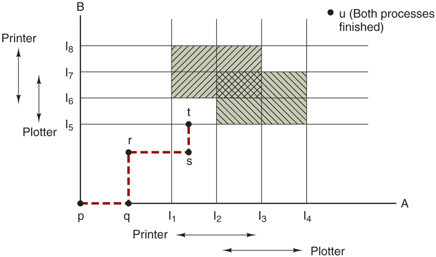
Two process resource trajectories.
Every point in the diagram represents a joint state of the two processes. Initially, the state is at p, with neither process having executed any instructions. If the scheduler chooses to run A first, we get to the point q, in which A has executed some number of instructions, but B has executed none. At point q the trajectory becomes vertical, indicating that the scheduler has chosen to run B. With a single processor, all paths must be horizontal or vertical, never diagonal. Furthermore, motion is always to the north or east, never to the south or west (because processes cannot run backward in time, of course).
When A crosses the line on the path from r to s, it requests and is granted the printer. When B reaches point t, it requests the plotter.
The regions that are shaded are especially interesting. The region with lines slanting from southwest to northeast represents both processes having the printer. The mutual exclusion rule makes it impossible to enter this region. Similarly, the region shaded the other way represents both processes having the plotter and is equally impossible.
If the system ever enters the box bounded by and on the sides and and top and bottom, it will eventually deadlock when it gets to the intersection of and At this point, A is requesting the plotter and B is requesting the printer, and both are already assigned. The entire box is unsafe and must not be entered. At point t the only safe thing to do is run process A until it gets to Beyond that, any trajectory to u will do.
The important thing to see here is that at point t, B is requesting a resource. The system must decide whether to grant it or not. If the grant is made, the system will enter an unsafe region and eventually deadlock. To avoid the deadlock, B should be suspended until A has requested and released the plotter.
6.5.2 Safe and Unsafe States
The deadlock avoidance algorithms that we will study use the information of Fig. 6-9. At any instant of time, there is a current state consisting of E, A, C, and R. A state is said to be safe if there is some scheduling order in which every process can run to completion even if all of them suddenly request their maximum number of resources immediately. It is easiest to illustrate this concept by an example using one resource. In Fig. 6-12(a) we have a state in which A has three instances of the resource but may need as many as nine eventually. B currently has two and may need four altogether, later. Similarly, C also has two but may need an additional five. A total of 10 instances of the resource exist, so with seven resources already allocated, three there are still free.
Figure 6-12
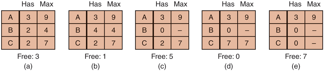
Demonstration that the state in (a) is safe.
The state of Fig. 6-12(a) is safe because there exists a sequence of allocations that allows all processes to complete execution. Namely, the scheduler can simply run B exclusively, until it asks for and gets two more instances of the resource, leading to the state of Fig. 6-12(b). When B completes, we get the state of Fig. 6-12(c). Then the scheduler can run C, leading eventually to Fig. 6-12(d). When C completes, we get Fig. 6-12(e). Now A can get the six instances of the resource it needs and also complete. Thus, the state of Fig. 6-12(a) is safe because the system, by careful scheduling, can avoid deadlock.
Now suppose we have the initial state shown in Fig. 6-13(a), but this time A requests and gets another resource, giving Fig. 6-13(b). Can we find a sequence that is guaranteed to work? Let us try. The scheduler could run B until it asked for all its resources, as shown in Fig. 6-13(c).
Figure 6-13
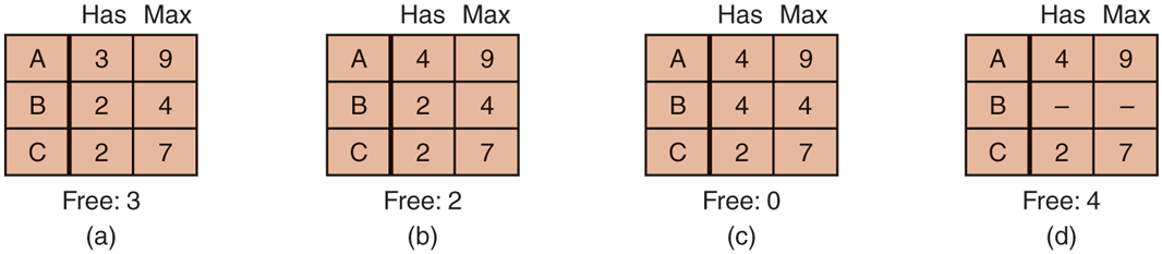
Demonstration that the state in (b) is not safe.
Eventually, B completes and we get the state of Fig. 6-13(d). At this point we are stuck. We only have four instances of the resource free, and each of the active processes needs five. There is no sequence that guarantees completion. Thus, the allocation decision that moved the system from Fig. 6-13(a) to Fig. 6-13(b) went from a safe to an unsafe state. Running A or C next starting at Fig. 6-13(b) does not work either. In retrospect, A’s request should not have been granted.
It is worth noting that an unsafe state is not a deadlocked state. Starting at Fig. 6-13(b), the system can run for a while. In fact, one process can even complete. Furthermore, it is possible that A might release a resource before asking for any more, allowing C to complete and avoiding deadlock altogether. Thus, the difference between a safe state and an unsafe state is that from a safe state the system can guarantee that all processes will finish; from an unsafe state, no such guarantee can be given.
6.5.3 The Banker’s Algorithm for a Single Resource
A scheduling algorithm that can avoid deadlocks is due to Dijkstra (1965); it is known as the banker’s algorithm and is an extension of the deadlock detection algorithm given in Sec. 6.5. It is modeled on the way a small-town banker might deal with a group of customers to whom he has granted lines of credit. (Years ago, banks did not lend money unless they knew they could be repaid.) What the algorithm does is check to see if granting the request leads to an unsafe state. If so, the request is denied. If granting the request leads to a safe state, it is carried out. In Fig. 6-14(a) we see four customers, A, B, C, and D, each of whom has been granted a certain number of credit units (e.g., 1 unit is 1K dollars). The banker knows that not all customers will need their maximum credit immediately, so he has reserved only 10 units rather than 22 to service them. (In this analogy, customers are processes, units are, say, printers, and the banker is the operating system.)
Figure 6-14
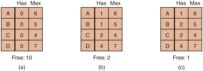
Three resource allocation states: (a) safe. (b) safe. (c) unsafe.
The customers go about their respective businesses, making loan requests from time to time (i.e., asking for resources). At a certain moment, the situation is as shown in Fig. 6-14(b). This state is safe because with two units left, the banker can delay any requests except C’s, thus letting C finish and release all four of his resources. With four units in hand, the banker can let either D or B have the necessary units, and so on.
Consider what would happen if a request from B for one more unit were granted in Fig. 6-14(b). We would have situation Fig. 6-14(c), which is unsafe. If all the customers suddenly asked for their maximum loans, the banker could not satisfy any of them, and we would have a deadlock. An unsafe state does not have to lead to deadlock, since a customer might not need the entire credit line available, but the banker cannot count on this behavior.
The banker’s algorithm considers each request as it occurs, seeing whether granting it leads to a safe state. If it does, the request is granted; otherwise, it is postponed until later. To see if a state is safe, the banker checks to see if he has enough resources to satisfy some customer. If so, those loans are assumed to be repaid, and the customer now closest to the limit is checked, and so on. If all loans can eventually be repaid, the state is safe and the initial request can be granted.
6.5.4 The Banker’s Algorithm for Multiple Resources
The banker’s algorithm can be generalized to handle multiple resources. Figure 6-15 shows how it works.
Figure 6-15
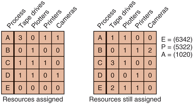
The banker’s algorithm with multiple resources.
In Fig. 6-15, we see two matrices. The one on the left shows how many of each resource are currently assigned to each of the five processes. The matrix on the right shows how many resources each process still needs in order to complete. These matrices are just C and R from Fig. 6-9. As in the single-resource case, processes must state their total resource needs before executing, so that the system can compute the right-hand matrix at each instant.
The three vectors at the right of the figure show the existing resources, E, the possessed resources, P, and the available resources, A, respectively. From E we see that the system has six tape drives, three plotters, four printers, and two cameras. Of these, five tape drives, three plotters, two printers, and two cameras are currently assigned. This fact can be seen by adding up the entries in the four resource columns in the left-hand matrix. The available resource vector is just the difference between what the system has and what is currently in use.
The algorithm for checking to see if a state is safe can now be stated.
Look for a row, R, whose unmet resource needs are all smaller than or equal to A. If no such row exists, the system will eventually deadlock since no process can run to completion (assuming processes keep all resources until they exit).
Assume the process of the chosen row requests all the resources it needs (which is guaranteed to be possible) and finishes. Mark that process as terminated and add all of its resources to the A vector.
Repeat steps 1 and 2 until either all processes are marked terminated (in which case the initial state was safe) or no process is left whose resource needs can be met (in which case the system was not safe).
If several processes are eligible to be chosen in step 1, it does not matter which one is selected: the pool of available resources either gets larger, or at worst, stays the same.
Now let us get back to the example of Fig. 6-15. The current state is safe. Suppose that process B now makes a request for the printer. This request can be granted because the resulting state is still safe (process D can finish, and then processes A or E, followed by the rest).
Now imagine that after giving B one of the two remaining printers, E wants the last printer. Granting that request would reduce the vector of available resources to (1 0 0 0), which leads to deadlock, so E’s request must be deferred for a while.
The banker’s algorithm was first published by Dijkstra in 1965. Since that time, nearly every book on operating systems has described it in detail. Innumerable papers have been written about various aspects of it. Unfortunately, few authors have had the audacity to point out that although in theory the algorithm is wonderful, in practice it is essentially useless because processes rarely know in advance what their maximum resource needs will be. In addition, the number of processes is not fixed, but dynamically varying as new users log in and out. Furthermore, resources that were thought to be available can suddenly vanish (tape drives can break). Thus, in practice, few, if any, existing systems use the banker’s algorithm for avoiding deadlocks. Some systems, however, use heuristics similar to those of the banker’s algorithm to prevent deadlock. For instance, networks may throttle traffic when buffer utilization reaches higher than, say, 70%—estimating that the remaining 30% will be sufficient for current users to complete their service and return their resources.