5.5 Clocks
Clocks (also called timers) are essential to the operation of any multiprogrammed system for a variety of reasons. They maintain the time of day and prevent one process from monopolizing the CPU, among other things. The clock software can take the form of a device driver, even though a clock is neither a block device, like a disk, nor a character device, like a mouse. Our examination of clocks will follow the same pattern as in the previous section: first a look at clock hardware and then a look at the clock software.
5.5.1 Clock Hardware
Two types of clocks are commonly used in computers, and both are quite different from the clocks and watches used by people. The simpler clocks are tied to the 110- or 220-volt power line and cause an interrupt on every voltage cycle, at 50 or 60 Hz. These clocks used to dominate, but are rare nowadays.
The other kind of clock is built out of three components: a crystal oscillator, a counter, and a holding register, as shown in Fig. 5-27. When a piece of quartz crystal is properly cut and mounted under tension, it can be made to generate a periodic signal of very great accuracy, typically in the range of several hundred megahertz to a few gigahertz, depending on the crystal chosen. Using electronics, this base signal can be multiplied by a small integer to get frequencies up to several gigahertz or even more. At least one such circuit is usually found in any computer, providing a synchronizing signal to the computer’s various circuits. This signal is fed into the counter to make it count down to zero. When the counter gets to zero, it causes a CPU interrupt.
Figure 5-27
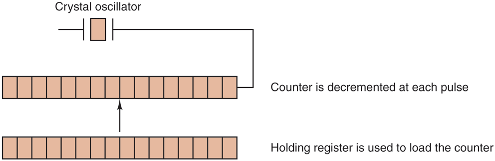
A programmable clock.
Programmable clocks typically have several modes of operation. In one-shot mode, when the clock is started, it copies the value of the holding register into the counter and then decrements the counter at each pulse from the crystal. When the counter gets to zero, it causes an interrupt and stops until it is explicitly started again by the software. In square-wave mode, after getting to zero and causing the interrupt, the holding register is automatically copied into the counter, and the whole process is repeated again indefinitely. These periodic interrupts are called clock ticks.
The advantage of the programmable clock is that its interrupt frequency can be controlled by software. If a 500-MHz crystal is used, then the counter is pulsed every 2 nsec. With (unsigned) 32-bit registers, interrupts can be programmed to occur at intervals from 2 nsec to 8.6 sec. Programmable clock chips usually contain two or three independently programmable clocks and have many other options as well (e.g., counting up instead of down, interrupts disabled, and more).
To prevent the current time from being lost when the computer’s power is turned off, most computers have a battery-powered backup clock, implemented with the kind of low-power circuitry used in digital watches. The battery clock can be read at startup. If the backup clock is not present, the software may ask the user for the current date and time. There is also a standard way for a networked system to get the current time from a remote host. In any case, the time is then translated into the number of clock ticks since 12 A.M. UTC (Universal Coordinated Time) (formerly known as Greenwich Mean Time) on January 1, 1970, as UNIX does, or since some other benchmark moment. The origin of time for Windows is January 1, 1980. At every clock tick, the real time is incremented by one count. Usually utility programs are provided to manually set the system clock and the backup clock and to synchronize the two clocks.
5.5.2 Clock Software
All the clock hardware does is generate interrupts at known intervals. Everything else involving time must be done by the software, the clock driver. The exact duties of the clock driver vary among operating systems, but usually include most of the following:
Maintaining the time of day.
Preventing processes from running longer than they are allowed to.
Accounting for CPU usage.
Handling the
alarmsystem call made by user processes.Providing watchdog timers for parts of the system itself.
Doing profiling, monitoring, and statistics gathering.
The first clock function, maintaining the time of day (also called the real time) is not difficult. It just requires incrementing a counter at each clock tick, as mentioned before. The only thing to watch out for is the number of bits in the time-of-day counter. With a clock rate of 60 Hz, a 32-bit counter will overflow in just over 2 years. Clearly the system cannot store the real time as the number of ticks since Jan. 1, 1970 in 32 bits.
Three approaches can be taken to solve this problem. The first way is to use a 64-bit counter, although doing so makes maintaining the counter more expensive since it has to be done many times a second. The second way is to maintain the time of day in seconds, rather than in ticks, using a subsidiary counter to count ticks until a whole second has been accumulated. Because seconds is more than 136 years, this method will work until the twenty-second century.
The third approach is to count in ticks, but to do that relative to the time the system was booted, rather than relative to a fixed external moment. When the backup clock is read or the user types in the real time, the system boot time is calculated from the current time-of-day value and stored in memory in any convenient form. Later, when the time of day is requested, the stored time of day is added to the counter to get the current time of day. All three approaches are shown in Fig. 5-28.
Figure 5-28
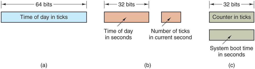
Three ways to maintain the time of day.
The second clock function is preventing processes from running too long. Whenever a process is started, the scheduler initializes a counter to the value of that process’ quantum in clock ticks. At every clock interrupt, the clock driver decrements the quantum counter by 1. When it gets to zero, the clock driver calls the scheduler to set up another process.
The third clock function is doing CPU accounting. The most accurate way to do it is to start a second timer, distinct from the main system timer, whenever a process is started up. When that process is stopped, the timer can be read out to tell how long the process has run. To do things right, the second timer should be saved when an interrupt occurs and restored afterward.
A less accurate, but simpler, way to do accounting is to maintain a pointer to the process table entry for the currently running process in a global variable. At every clock tick, a field in the current process’ entry is incremented. In this way, every clock tick is ‘‘charged’’ to the process running at the time of the tick. A minor problem with this strategy is that if many interrupts occur during a process’ run, it is still charged for a full tick, even though it did not get much work done. Properly accounting for the CPU during interrupts is too expensive and is rarely done.
In many systems, a process can request that the operating system give it a warning after a certain interval. The warning is usually a signal, interrupt, message, or something similar. One application requiring such warnings is networking, in which a packet not acknowledged within a certain time interval must be retransmitted. Another application is computer-aided instruction, where a student not providing a response within a certain time is told the answer.
If the clock driver had enough clocks, it could set a separate clock for each request. This not being the case, it must simulate multiple virtual clocks with a single physical clock. One way is to maintain a table in which the signal time for all pending timers is kept, as well as a variable giving the time of the next one. Whenever the time of day is updated, the driver checks to see if the closest signal has occurred. If it has, the table is searched for the next one to occur.
If many signals are expected, it is more efficient to simulate multiple clocks by chaining all the pending clock requests together, sorted on time, in a linked list, as shown in Fig. 5-29. Each entry on the list tells how many clock ticks following the previous one to wait before causing a signal. In this example, signals are pending for 4203, 4207, 4213, 4215, and 4216.
Figure 5-29
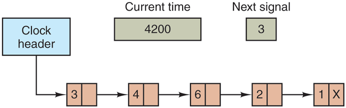
Simulating multiple timers with a single clock.
In Fig. 5-29, the next interrupt occurs in 3 ticks. On each tick, Next signal is decremented. When it gets to 0, the signal corresponding to the first item on the list is caused, and that item is removed from the list. Then Next signal is set to the value in the entry now at the head of the list, in this example, 4.
Note that during a clock interrupt, the clock driver has several things to do— increment the real time, decrement the quantum and check for 0, do CPU accounting, and decrement the alarm counter. However, each of these operations has been carefully arranged to be very fast because they have to be repeated many times a second.
Parts of the operating system also need to set timers. These are called watchdog timers and are frequently used (especially in embedded devices) to detect problems such as hangs. For instance, a watchdog timer may reset a system that stops running. While the system is running, it regularly resets the timer, so that it never expires. In that case, expiration of the timer proves that the system has not run for a long time, and leads to corrective action—such as a full-system reset.
The mechanism used by the clock driver to handle watchdog timers is the same as for user signals. The only difference is that when a timer goes off, instead of causing a signal, the clock driver calls a procedure supplied by the caller. The procedure is part of the caller’s code. The called procedure can do whatever is necessary, even causing an interrupt, although within the kernel interrupts are often inconvenient and signals do not exist. That is why the watchdog mechanism is provided. It is worth nothing that the watchdog mechanism works only when the clock driver and the procedure to be called are in the same address space.
The last thing in our list is profiling. Some operating systems provide a mechanism by which a user program can have the system build up a histogram of its program counter, so it can see where it is spending its time. When profiling is a possibility, at every tick the driver checks to see if the current process is being profiled, and if so, computes the bin number (a range of addresses) corresponding to the current program counter. It then increments that bin by one. This mechanism can also be used to profile the system itself.
5.5.3 Soft Timers
Most computers have a second programmable clock that can be set to cause timer interrupts at whatever rate a program needs. This timer is in addition to the main system timer whose functions were described above. As long as the interrupt frequency is low, there is no problem using this second timer for application-specific purposes. The trouble arrives when the frequency of the application-specific timer is very high. Below we will briefly describe a software-based timer scheme that works well under many circumstances, even at fairly high frequencies. The idea is due to Aron and Druschel (1999). For more details, please see their paper.
Generally, there are two ways to manage I/O: interrupts and polling. Interrupts have low latency, that is, they happen immediately after the event itself with little or no delay. On the other hand, with modern CPUs, interrupts have a substantial overhead due to the need for context switching and their influence on the pipeline, TLB, and cache.
The alternative to interrupts is to have the application poll for the event expected itself. Doing this avoids interrupts, but there may be substantial latency because an event may happen directly after a poll, in which case it waits almost a whole polling interval. On the average, the latency is half the polling interval.
Interrupt latency today is barely better than that of computers in the 1970s. On most minicomputers, for example, an interrupt took four bus cycles: to stack the program counter and PSW and to load a new program counter and PSW. Nowadays, dealing with the pipeline, MMU, TLB, and cache adds a great deal of time to the overhead. These effects are likely to get worse rather than better in time, thus canceling out faster clock rates. Unfortunately, for certain applications, we want neither the overhead of interrupts nor the latency of polling.
Soft timers avoid interrupts. Instead, whenever the kernel is running for some other reason, just before it returns to user mode it checks the real-time clock to see if a soft timer has expired. If it has expired, the scheduled event (e.g., packet transmission or checking for an incoming packet) is performed, with no need to switch into kernel mode since the system is already there. After the work has been performed, the soft timer is reset to go off again. All that has to be done is copy the current clock value to the timer and add the timeout interval to it.
Soft timers stand or fall with the rate at which kernel entries are made for other reasons. These reasons include the following:
System calls.
TLB misses.
Page faults.
I/O interrupts.
The CPU going idle.
To see how often these events happen, Aron and Druschel made measurements with several CPU loads, including a fully loaded Web server, a Web server with a compute-bound background job, playing real-time audio from the Internet, and recompiling the UNIX kernel. The average entry rate into the kernel varied from 2 to with about half of these entries being system calls. Thus to a first-order approximation, having a soft timer go off, say, every is doable, albeit with an occasional missed deadline. Being late from time to time is often better than having interrupts eat up 35% of the CPU.
Of course, there will be periods when there are no system calls, TLB misses, or page faults, in which case no soft timers will go off. To put an upper bound on these intervals, the second hardware timer can be set to go off, say, every 1 msec. If the application can live with only 1000 activations per second for occasional intervals, then the combination of soft timers and a low-frequency hardware timer may be better than either pure interrupt-driven I/O or pure polling.