5.4 Mass Storage: Disk and SSD
Now we will begin studying some real I/O devices. We will begin with storage devices. In later sections, we examine clocks, keyboards, and displays. Modern storage devices come in a variety of types. The most common ones are magnetic hard disks and SSDs. For distribution of programs, data, and movies, old fogeys may still use optical disks (DVDs and Blu-ray), but these are rapidly going out of fashion and will not be discussed in this (undeniably fashionable) book. Instead, we briefly discuss magnetic disks and SSDs. We will start with the former, as it is a nice case study.
5.4.1 Magnetic Disks
Magnetic disks are characterized by the fact that reads and writes are equally fast, which makes them suitable as secondary memory (paging, file systems, etc.). Arrays of these disks are sometimes used to provide highly reliable storage. They are organized into cylinders, each one containing as many tracks as there are heads stacked vertically. The tracks are divided into sectors, with typically up to several hundreds of sectors around the circumference. The number of heads varies from 1 to about 16.
Older disks had little electronics and just delivered a simple serial bit stream. On these disks, the controller did most of the work. On other disks, in particular, SATA (Serial ATA) disks, the drive itself contains a microcontroller that does considerable work and allows the real disk controller to issue a set of higher-level commands. The controller does track caching, bad-block remapping, and more.
A device feature that has important implications for the disk driver is the possibility of a controller doing seeks on two or more drives at the same time. These are known as overlapped seeks. While the controller and software are waiting for a seek to complete on one drive, the controller can initiate a seek on another drive. Many controllers can also read or write on one drive while seeking on one or more other drives. Moreover, a system with several hard disks with integrated controllers can operate them simultaneously, at least to the extent of transferring between the disk and the controller’s buffer memory. However, only one transfer between the controller and the main memory is possible at once. The ability to perform two or more operations at the same time can reduce the average access time considerably.
If we compare the standard storage medium of the original IBM PC (a floppy disk) with a modern hard disk, such as the Seagate IronWolf Pro, we see that many things have changed. First, the disk capacity of the old floppy disk was 360 KB, or about one third of the capacity needed to store the PDF of just this chapter. In contrast, the IronWolf packs as much as 18 TB—an increase of give or take 8 orders of magnitude. The authors solemnly promise never to make the chapter that big. The transfer rate also went up from around 23 KB/sec to 250 MB/sec, a jump of 4 orders of magnitude. The latency, however, improved more marginally, from around 100 msec to 4 msec. Better, but you may find it a bit underwhelming.
One thing to be aware of in looking at the specifications of modern hard disks is that the geometry specified, and used by the driver software, is almost always different from the physical format. On old disks, the number of sectors per track was the same for all cylinders. For instance, the IBM PC floppy disk had 9 sectors of 512 bytes on every track. Modern disks, on the other hand, are divided into zones with more sectors on the outer zones than the inner ones. Figure 5-18(a) illustrates a tiny disk with two zones. The outer zone has 32 sectors per track; the inner one has 16 sectors per track. A real disk easily has tens of zones, with the number of sectors increasing per zone as one goes out from the innermost to the outermost zone.
Figure 5-18
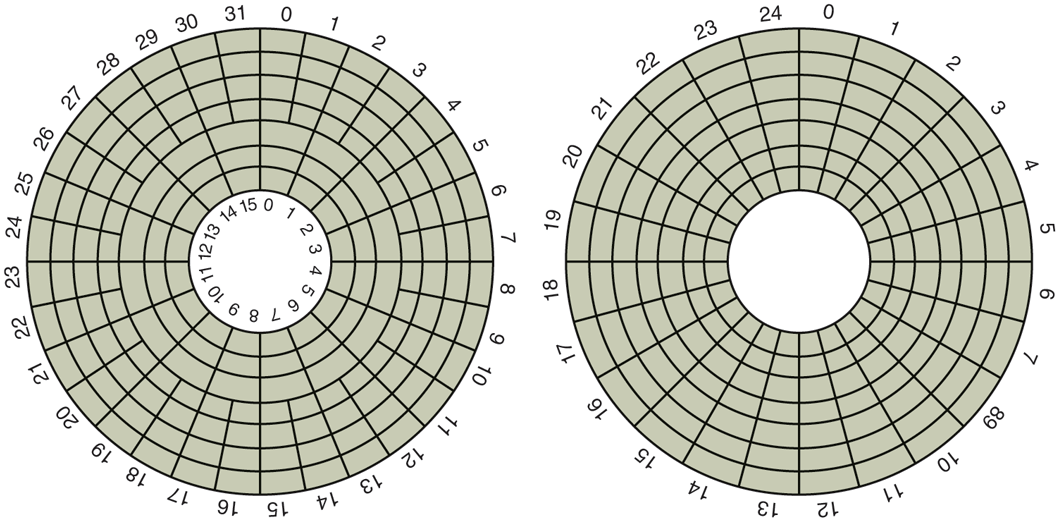
(a) Physical geometry of a disk with two zones. (b) A possible virtual geometry for this disk.
To hide the details of how many sectors each track has, most modern disks have a virtual geometry that is presented to the operating system. The software is instructed to act as though there are x cylinders, y heads, and z sectors per track. The controller then remaps a request for (x, y, z) onto the real cylinder, head, and sector. A possible virtual geometry for the physical disk of Fig. 5-18(a) is shown in Fig. 5-18(b). In both cases, the disk has 192 sectors, only the published arrangement is different than the real one. Simplifying the addressing even more, modern disks now support a system called logical block addressing, in which disk sectors are just numbered consecutively starting at 0, without regard to the disk geometry.
Disk Formatting
A hard disk consists of a stack of aluminum, alloy, or glass platters typically 3.5 inch in diameter (or 2.5 inch on notebook computers). On each platter is deposited a thin magnetizable metal oxide. After manufacturing, there is no information whatsoever on the disk.
Before the disk can be used, each platter must receive a low-level format done by software. The format consists of a series of concentric tracks, each containing some number of sectors, with short gaps between the sectors. The format of a sector is shown in Fig. 5-19.
Figure 5-19

A disk sector.
The preamble starts with a certain bit pattern that allows the hardware to recognize the start of the sector. It also contains the cylinder and sector numbers and some other information. The size of the data portion is determined by the low-level formatting program. Most disks use 512-byte sectors. The ECC field contains redundant information that can be used to recover from read errors. The size and content of this field varies from manufacturer to manufacturer, depending on how much disk space the designer is willing to give up for higher reliability and how complex an ECC code the controller can handle. A 16-byte ECC field is not unusual. Furthermore, all hard disks have some number of spare sectors allocated to be used to replace sectors with a manufacturing defect.
The position of sector 0 on each track is offset from the previous track when the low-level format is laid down. This offset, called cylinder skew, is done to improve performance. The idea is to allow the disk to read multiple tracks in one continuous operation without losing data. The nature of the problem can be seen by looking at Fig. 5-18(a). Suppose that a request needs 18 sectors starting at sector 0 on the innermost track. Reading the first 16 sectors takes one disk rotation, but a seek is needed to move outward one track to get the 17th sector. By the time the head has moved one track, sector 0 has rotated past the head so an entire rotation is needed until it comes by again. That problem is eliminated by offsetting the sectors as shown in Fig. 5-20.
Figure 5-20
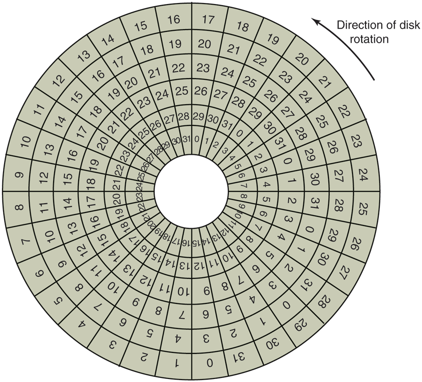
An illustration of cylinder skew.
The amount of cylinder skew depends on the drive geometry. For example, a 10,000-RPM (Revolutions Per Minute) drive rotates in 6 msec. If a track contains 300 sectors, a new sector passes under the head every If the track-to-track seek time is 40 sectors will pass by during the seek, so the cylinder skew should be at least 40 sectors, rather than the three sectors shown in Fig. 5-20. It is worth mentioning that switching between heads also takes a finite time, so there is head skew as well as cylinder skew, but head skew is not very large, usually much less than one sector time.
As a result of the low-level formatting, disk capacity is reduced, depending on the sizes of the preamble, intersector gap, and ECC, as well as the number of spare sectors reserved. Often the formatted capacity is 20% lower than the unformatted capacity. The spare sectors do not count toward the formatted capacity, so all disks of a given type have exactly the same capacity when shipped, independent of how many bad sectors they actually have (if the number of bad sectors exceeds the number of spares, the drive will be rejected and not shipped).
There is considerable confusion about disk capacity because some manufacturers advertised the unformatted capacity to make their drives look larger than they in reality are. For example, let us consider a drive whose unformatted capacity is bytes. This might be sold as a 20-TB disk. However, after formatting, possibly only bytes are available for data. To add to the confusion, the operating system may report this capacity as 15 TB, not 17 TB, because software considers a memory of 1 TB to be (1.099.511.627.776) bytes, not (1,000,000,000,000) bytes. It would be better if this were reported as 15 TiB.
To make things even worse, in the world of data communications, 1 Tbps means 1,000,000,000,000 bits/sec because the prefix Tera really does mean (a kilometer is 1000 meters, not 1024 meters, after all). Only with memory and disk sizes do kilo, mega, giga, tera, peta, exa, and zetta mean and respectively.
To avoid confusion, some authors use the prefixes kilo, mega, giga, tera, peta, exa, and zetta to mean and respectively, while using kibi, mebi, gibi, tebi, pebi, exbi, and zebi to mean etc. However, the use of the ‘‘b’’ prefixes is relatively rare. Just in case you like really big numbers, one yottabyte is and a yobibyte bytes.
Formatting also affects performance. If a track on a 10,000-RPM disk has 300 sectors of 512 bytes each, it takes 6 msec to read the 153,600 bytes on the track for a data rate of 25,600,000 bytes/sec or 24.4 MB/sec. It is not possible to go faster than this, no matter what kind of interface is present, even if it is a SATA interface at 6 GB/sec.
Actually reading continuously at this rate requires a large buffer in the controller. Consider, for example, a controller with a one-sector buffer that has been given a command to read two consecutive sectors. After reading the first sector from the disk and doing the ECC calculation, the data must be transferred to main memory. While this transfer is taking place, the next sector will fly by the head. When the copy to memory is complete, the controller will have to wait almost an entire rotation time for the second sector to come around again.
This problem can be eliminated by numbering the sectors in an interleaved fashion when formatting the disk. In Fig. 5-21(a), we see the usual numbering pattern (ignoring cylinder skew here). In Fig. 5-21(b), we see single interleaving, which gives the controller some breathing space between consecutive sectors in order to copy the buffer to main memory.
Figure 5-21
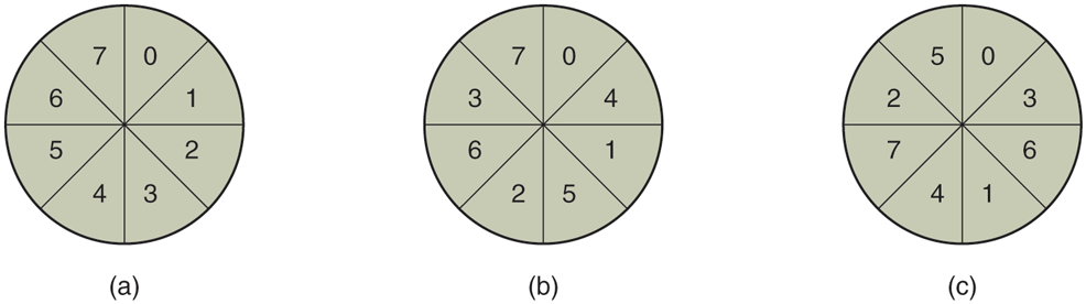
(a) No interleaving. (b) Single interleaving. (c) Double interleaving.
If the copying process is very slow, the double interleaving of Fig. 5-22(c) may be needed. If the controller has a buffer of only one sector, it does not matter whether the copying from the buffer to main memory is done by the controller, the main CPU, or even a DMA chip; it still takes some time. To avoid the need for interleaving, the controller should be able to buffer an entire track. With hundreds of MB of memory, most modern controllers can buffer many entire tracks.
After low-level formatting is completed, the disk is partitioned. Logically, each partition is like a separate disk. Partitions are needed to allow multiple operating systems to coexist. Also, in some cases, a partition can be used for swapping. In older other computers, sector 0 contains the MBR (Master Boot Record), which contains some boot code plus the partition table at the end. The MBR, and thus support for partition tables, first appeared in IBM PCs in 1983 to support the then massive 10-MB hard drive in the PC XT. Disks have grown a bit since then. As MBR partition entries in most systems are limited to 32 bits, the maximum disk size that can be supported with 512 B sectors is 2 TB. For this reason, most operating since now also support the new GPT (GUID Partition Table), which supports disk sizes up to 9.4 ZB (9,444,732,965,739,290,426,880 bytes or some 8 ZiB). At the time this book went to press, this was considered a lot of bytes.
The partition table gives the starting sector and size of each partition. You can see more about the GPT in UEFI in Sec. 4.3. If there are four partitions and all of them are for Windows, they will be called C:, D:, E:, and F: and treated as separate drives. If three of them are for Windows and one is for UNIX, then Windows will call its partitions C:, D:, and E:. If a USB drive is added, it will be F:. To be able to boot from the hard disk, one partition must be marked as active in the partition table.
The final step in preparing a disk for use is to perform a high-level format of each partition (separately). This operation lays down a boot block, the free storage administration (free list or bitmap), root directory, and an empty file system. It also puts a code in the partition table entry telling which file system is used in the partition because many operating systems support multiple incompatible file systems (for historical reasons). At this point the system can be booted.
We already saw in Chap. 1 that when the power is turned on, the BIOS runs initially and reads the GPT. It then finds the appropriate bootloader and executes i to boot the operating system.
Disk Arm Scheduling Algorithms
In this section, we will look at some issues related to disk drivers in general. First, consider how long it takes to read or write a disk block. The time required is determined by three factors:
Seek time (the time to move the arm to the proper cylinder).
Rotational delay (how long for the proper sector to appear under the reading head).
Actual data transfer time.
For most disks, the seek time dominates the other two times, so reducing the mean seek time can improve system performance substantially.
If the disk driver accepts requests one at a time and carries them out in that order, that is, FCFS (First-Come, First-Served), little can be done to optimize seek time. However, another strategy is possible when the disk is heavily loaded. It is likely that while the arm is seeking on behalf of one request, other disk requests may be generated by other processes. Many disk drivers maintain a table, indexed by cylinder number, with all the pending requests for each cylinder chained together in a linked list headed by the table entries.
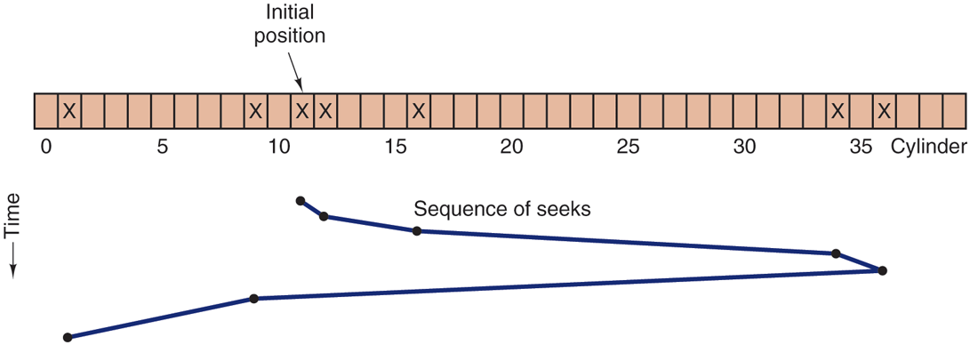
Given this kind of data structure, we can improve upon the first-come, first served scheduling algorithm. To see how, consider an imaginary disk with 40 cylinders. A request comes in to read a block on cylinder 11. While the seek to cylinder 11 is in progress, new requests come in for cylinders 1, 36, 16, 34, 9, and 12, in that order. They are entered into the table of pending requests, with a separate linked list for each cylinder. The requests are shown in Fig. 5-22.
Figure 5-22
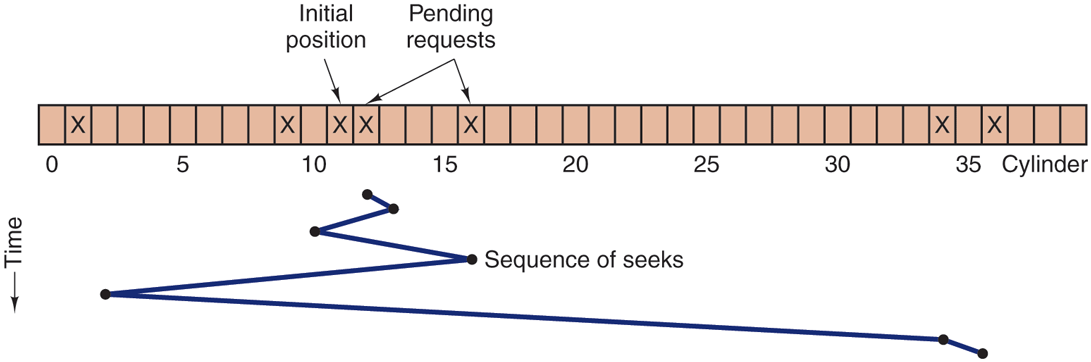
Shortest Seek First (SSF) disk scheduling algorithm.
When the current request (for cylinder 11) is finished, the disk driver has a choice of which request to handle next. Using FCFS, it would go next to cylinder 1, then to 36, and so on. This algorithm would require arm motions of 10, 35, 20, 18, 25, and 3, respectively, for a total of 111 cylinders.
Alternatively, it could always handle the closest request next, to minimize seek time. Given the requests of Fig. 5-22, the sequence is 12, 9, 16, 1, 34, and 36, shown as the jagged line at the bottom of Fig. 5-22. With this sequence, the arm motions are 1, 3, 7, 15, 33, and 2, for a total of 61 cylinders. This algorithm, called SSF (Shortest Seek First), cuts the total arm motion almost in half versus FCFS.
Unfortunately, SSF has a problem. Suppose more requests keep coming in while the requests of Fig. 5-22 are being processed. For example, if, after going to cylinder 16, a new request for cylinder 8 is present, that request will have priority over cylinder 1. If a request for cylinder 13 then comes in, the arm will next go to 13, instead of 1. With a heavily loaded disk, the arm will tend to stay in the middle of the disk most of the time, so requests at either extreme will have to wait until a statistical fluctuation in the load causes there to be no requests near the middle. Requests far from the middle may get poor service. The goals of minimal response time and fairness are in conflict here.
Tall buildings also have to deal with this trade-off. The problem of scheduling an elevator in a tall building is similar to that of scheduling a disk arm. Requests come in continuously calling the elevator to floors (cylinders) at random. The computer running the elevator could easily keep track of the sequence in which customers pushed the call button and service them using FCFS or SSF.
However, most elevators use a different algorithm in order to reconcile the mutually conflicting goals of efficiency and fairness. They keep moving in the same direction until there are no more outstanding requests in that direction, then they switch directions. This algorithm, known both in the disk world and the elevator world as the elevator algorithm, requires the software to maintain 1 bit: the current direction bit, UP or DOWN. When a request finishes, the disk or elevator driver checks the bit. If it is UP, the arm or cabin is moved to the next highest pending request. If no requests are pending at higher positions, the direction bit is reversed. When the bit is set to DOWN, the move is to the next lowest requested position, if any. If no request is pending, it just stops and waits. In big office towers, when there are no requests pending, the software might send the cabin to the ground floor, since it is more likely to be need there shortly than on, say, the 19th floor. Disk software does not usually try to speculatively preposition the head anywhere.
Figure 5-23 shows the elevator algorithm using the same seven requests as Fig. 5-22, assuming the direction bit was initially UP. The order in which the cylinders are serviced is 12, 16, 34, 36, 9, and 1, which yields arm motions of 1, 4, 18, 2, 27, and 8, for a total of 60 cylinders. In this case, the elevator algorithm is slightly better than SSF, although it is usually worse. One nice property the elevator algorithm has is that given any collection of requests, the upper bound on the total motion is fixed: it is just twice the number of cylinders.
Figure 5-23
The elevator algorithm for scheduling disk requests.
A slight modification of this algorithm that has a smaller variance in response times (Teory, 1972) is to always scan in the same direction. When the highest-numbered cylinder with a pending request has been serviced, the arm goes to the lowest-numbered cylinder with a pending request and then continues moving in an upward direction. In effect, the lowest-numbered cylinder is thought of as being just above the highest-numbered cylinder.
Some disk controllers provide a way for the software to inspect the current sector number under the head. With such a controller, another optimization is possible. If two or more requests for the same cylinder are pending, the driver can issue a request for the sector that will pass under the head next. Note that when multiple tracks are present in a cylinder, consecutive requests can be for different tracks with no penalty. The controller can select any of its heads almost instantaneously (head selection involves neither arm motion nor rotational delay).
If the disk has the property that seek time is much faster than the rotational delay, then a different optimization should be used. Pending requests should be sorted by sector number, and as soon as the next sector is about to pass under the head, the arm should be zipped over to the right track to read or write it.
With a modern hard disk, the seek and rotational delays so dominate performance that reading one or two sectors at a time is very inefficient. For this reason, many disk controllers always read and cache multiple sectors, even when only one is requested. Typically any request to read a sector will cause that sector and much or all the rest of the current track to be read, depending upon how much space is available in the controller’s cache memory. The Seagate IronWolf hard disk described earlier has a 256-MB cache, for example. The use of the cache is determined dynamically by the controller. In the simplest case, the cache is divided into two sections, one for reads and one for writes. If a subsequent read can be satisfied out of the controller’s cache, it can return the requested data immediately.
It is worth noting that the disk controller’s cache is completely independent of the operating system’s cache. The controller’s cache usually holds blocks that have not actually been requested, but which were convenient to read because they just happened to pass under the head as a side effect of some other read. In contrast, any cache maintained by the operating system will consist of blocks that were explicitly read and which the operating system thinks might be needed again in the near future (e.g., a disk block holding a directory block).
When several drives are present on the same controller, the operating system should maintain a pending request table for each drive separately. Whenever any drive is idle, a seek should be issued to move its arm to the cylinder where it will be needed next (assuming the controller allows overlapped seeks). When the current transfer finishes, a check can be made to see if any drives are positioned on the correct cylinder. If one or more are, the next transfer can be started on a drive that is already on the right cylinder. If none of the arms is in the right place, the driver should issue a new seek on the drive that just completed a transfer and wait until the next interrupt to see which arm gets to its destination first.
It is important to realize that all of the above disk-scheduling algorithms tacitly assume that the real disk geometry is the same as the virtual geometry. If it is not, then scheduling disk requests makes no sense because the operating system cannot really tell whether cylinder 40 or cylinder 200 is closer to cylinder 39. On the other hand, if the disk controller can accept multiple outstanding requests, it can use these scheduling algorithms internally. In that case, the algorithms are still valid, but one level down, inside the controller.
Error Handling
Disk manufacturers are constantly pushing the limits of the technology by increasing linear bit densities. The IronWolf hard disk of our examples packs as many a 2470 Kbits per inch on average. Recording that many bits per inch requires an extremely uniform substrate and a very fine oxide coating. Unfortunately, it is not possible to manufacture a disk to such specifications without defects. As soon as manufacturing technology has improved to the point where it is possible to operate flawlessly at such densities, disk designers will go to higher densities to increase the capacity. Doing so will probably reintroduce defects.
Manufacturing defects introduce bad sectors, that is, sectors that do not correctly read back the value just written to them. If the defect is very small, say, only a few bits, it is possible to use the bad sector and just let the ECC correct the errors every time. If the defect is bigger, the error cannot be masked.
There are two general approaches to bad blocks: deal with them in the controller or deal with them in the operating system. In the former approach, before the disk is shipped from the factory, it is tested and a list of bad sectors is written onto the disk. For each bad sector, one of the spares is substituted for it.
There are two ways to do this substitution. In Fig. 5-24(a), we see a single disk track with 30 data sectors and two spares. Sector 7 is defective. What the controller can do is remap one of the spares as sector 7 as shown in Fig. 5-24(b). The other way is to shift all the sectors up one, as shown in Fig. 5-24(c). In both cases the controller has to know which sector is which. It can keep track of this information through internal tables (one per track) or by rewriting the preambles to give the remapped sector numbers. If the preambles are rewritten, the method of Fig. 5-24(c) is more work (because 23 preambles must be rewritten) but ultimately gives better performance because an entire track can still be read in one rotation.
Figure 5-24
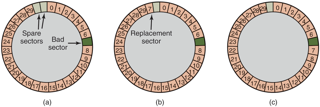
(a) A disk track with a bad sector. (b) Substituting a spare for the bad sector. (c) Shifting all the sectors to bypass the bad one.
Errors can also develop during normal operation after the drive has been installed. The first line of defense upon getting an error that the ECC cannot handle is to just try the read again. Some read errors are transient, that is, are caused by specks of dust under the head and will go away on a second attempt. If the controller notices that it is getting repeated errors on a certain sector, it can switch to a spare before the sector has died completely. In this way, no data are lost and the operating system and user do not even notice the problem. Usually, the method of Fig. 5-24(b) has to be used since the other sectors might now contain data. Using the method of Fig. 5-24(c) would require not only rewriting the preambles, but copying all the data as well.
Earlier we said there were two general approaches to handling errors: handle them in the controller or in the operating system. If the controller does not have the capability to transparently remap sectors as we have discussed, the operating system must do the same thing in software. This means that it must first acquire a list of bad sectors, either by reading them from the disk, or simply testing the entire disk itself. Once it knows which sectors are bad, it can build remapping tables. If the operating system wants to use the approach of Fig. 5-24(c), it must shift the data in sectors 7 through 29 up one sector.
If the operating system is handling the remapping, it must make sure that bad sectors do not occur in any files and also do not occur in the free list or bitmap. One way to do this is to create a secret file consisting of all the bad sectors. If this file is not entered into the file system, users will not accidentally read it (or worse yet, free it).
However, there is still another problem: backups. If the disk is backed up file by file, it is important that the backup utility not try to copy the bad block file. To prevent this, the operating system has to hide the bad block file so well that even a backup utility cannot find it. If the disk is backed up sector by sector rather than file by file, it will be difficult, if not impossible, to prevent read errors during backup. The only hope is that the backup program has enough smarts to give up after 10 failed reads and continue with the next sector.
Bad sectors are not the only source of errors. Seek errors caused by mechanical problems in the arm also occur. The controller keeps track of the arm position internally. To perform a seek, it issues a command to the arm motor to move the arm to the new cylinder. When the arm gets to its destination, the controller reads the actual cylinder number from the preamble of the next sector. If the arm is in the wrong place, a seek error has occurred.
Most hard disk controllers correct seek errors automatically, but most of the old floppy controllers used in the 1980s and 1990s just set an error bit and left the rest to the driver. The driver handled this error by issuing a recalibrate command, to move the arm as far out as it would go and reset the controller’s internal idea of the current cylinder to 0. Usually this solved the problem. If it did not, the drive had to be repaired.
As we have just seen, the controller is really a specialized little computer, complete with software, variables, buffers, and occasionally, bugs. Sometimes an unusual sequence of events, such as an interrupt on one drive occurring simultaneously with a recalibrate command for another drive will trigger a bug and cause the controller to go into a loop or lose track of what it was doing. Controller designers usually plan for the worst and provide a pin on the chip which, when asserted, forces the controller to forget whatever it was doing and reset itself. If all else fails, the disk driver can set a bit to invoke this signal and reset the controller. If that does not help, all the driver can do is print a message and give up.
Recalibrating a disk makes a funny noise but otherwise normally is not disturbing. However, there is one situation where recalibration is a problem: systems with real-time constraints. When a video is being played off (or served from) a hard disk, or files from a hard disk are being burned onto a Blu-ray disc, it is essential that the bits arrive from the hard disk at a uniform rate. Under these circumstances, recalibrations insert gaps into the bit stream and are unacceptable. Special drives, called AV disks (Audio Visual disks), which never recalibrate are available for such applications.
Anecdotally, a highly convincing demonstration of how advanced disk controllers have become was given by the Dutch hacker Jeroen Domburg, who hacked a modern disk controller to make it run custom code. It turns out the disk controller is equipped with a fairly powerful multicore ARM processor and has easily enough resources to run Linux. If the bad guys hack your hard drive in this way, they will be able to see and modify all data you transfer to and from the disk. Even reinstalling the operating from scratch will not remove the infection, as the disk controller itself is malicious and serves as a permanent backdoor. Alternatively, you can collect a stack of broken hard drives from your local recycling center and build your own cluster computer for free.
5.4.2 Solid State Drives (SSDs)
As we saw in Sec. 4.3.7, SSDs are fast, have asymmetric read and write performance, and contain no moving parts. They come in different guises. For instance, there are some that conform to the SATA standard for storage devices that is also used for magnetic disks. However, since SATA was designed for mechanical disks that are slow compared to flash technology, more and more SSDs now interface to the rest of the system using NVMe (Non-Volatile Memory Express). NVMe is a standard to exploit better the speed of the fast PCI Express connection between the SSD and the rest of the system, as well as the parallelism available in the SSD itself.
For instance, since modern computers have multiple cores and the SSD consists of many (flash) pages, blocks and, ultimately, chips, it pays off to process requests in parallel. To make this possible, NVMe supports multiple queues. At the very least, NVMe offers one command request queue (known as a submission queue in NVMe terminology) and one reply queue (known as a completion queue) per core. To perform storage requests, a core will first write I/O commands in its request queue and then write to the doorbell register when the commands are ready to execute. The doorbell triggers the controller on the SSD to process the entries in some order (e.g., in the order in which they were received, or in order of priority). When the request completes, it will write the result as a status code in the reply queue.
NVMe queues have multiple advantages. First, where SATA offers only a single queue with a small number of entries, NVMe allows many (and longer) queues—up to 64K queues with up to 64K I/O commands entries each. Each queue is processed in parallel, thus allowing the controller to push more commands to the flash chips and speeding up the storage I/O significantly. Second, because of this, since the overall computer system now needs fewer devices to support the same number of I/O operations, this also reduces the power and cooling requirements. As a bonus, NVMe allows file systems more direct access to the PCIe bus† and SSD, meaning that fewer layers of software are involved in NVMe than in SATA operations.
If our SSD uses NVMe, the operating system needs a driver for NVMe also. Often, this driver in turn consists of multiple components, such as a module that is more or less hardware independent, a module specifically for PCIe, a module for TCP, etc. This is not uncommon and drivers often consist of a number of logical components. The good news here is that the SSD interface is standardized by NVMe, and so the operating system needs only a single driver to handle all conforming SSDs. Nowadays, all major operating systems provide support for NVMe, and thus for NVMe SSDs.
Stable Storage
As we have seen, disks sometimes make errors. Good sectors can suddenly become bad sectors. Whole drives can die unexpectedly. For some applications, it is essential that data never be lost or corrupted, even in the face of disk and CPU errors. Ideally, a disk should simply work all the time with no errors. Unfortunately, that is not achievable. What is achievable is a disk subsystem that has the following property: when a write is issued to it, the disk either correctly writes the data or it does nothing, leaving the existing data intact. Such a system is called stable storage and is implemented in software (Lampson and Sturgis, 1979). The goal is to keep the disk consistent at all costs. Below we will describe a slight variant of the original idea.
Before describing the algorithm, it is important to have a clear model of the possible errors. The model assumes that when a disk writes a block (one or more sectors), either the write is correct or it is incorrect and this error can be detected on a subsequent read by examining the values of the ECC fields. In principle, guaranteed error detection is never possible because with a, say, 16-byte ECC field guarding a 512-byte sector, there are data values and only ECC values. Thus if a block is garbled during writing but the ECC is not, there are billions upon billions of incorrect combinations that yield the same ECC. If any of them occur, the error will not be detected. On the whole, the probability of random data having the proper 16-byte ECC is about which is small enough that we will call it zero, even though it is really not.
The model also assumes that a correctly written sector can spontaneously go bad and become unreadable. However, the assumption is that such events are so rare that having the same sector go bad on a second (independent) drive during a reasonable time interval (e.g., 1 day) is small enough to ignore.
The model also assumes the CPU can fail, in which case it just stops. Any disk write in progress at the moment of failure also stops, leading to incorrect data in one sector and an incorrect ECC that can later be detected. Under all these conditions, stable storage can be made 100% reliable in the sense of writes either working correctly or leaving the old data in place. Of course, it does not protect against physical disasters, such as an earthquake happening and the computer falling 100 meters into a fissure and landing in a pool of boiling magma. It is tough to recover from this condition in software.
Stable storage uses a pair of identical disks with the corresponding blocks working together to form one error-free block. In the absence of errors, the corresponding blocks on both drives are the same. Either one can be read to get the same result. To achieve this goal, the following three operations are defined:
Stable writes. A stable write consists of first writing the block on drive 1, then reading it back to verify that it was written correctly. If it was not, the write and reread are done again up to n times until they work. After n consecutive failures, the block is remapped onto a spare and the operation repeated until it succeeds, no matter how many spares have to be tried. After the write to drive 1 has succeeded, the corresponding block on drive 2 is written and reread, repeatedly if need be, until it, too, finally succeeds. In the absence of CPU crashes, when a stable write completes, the block has correctly been written onto both drives and verified on both of them.
Stable reads. A stable read first reads the block from drive 1. If this yields an incorrect ECC, the read is tried again, up to n times. If all of these give bad ECCs, the corresponding block is read from drive 2. Given the fact that a successful stable write leaves two good copies of the block behind, and our assumption that the probability of the same block spontaneously going bad on both drives in a reasonable time interval is negligible, a stable read always succeeds.
Crash recovery. After a crash, a recovery program scans both disks comparing corresponding blocks. If a pair of blocks are both good and the same, nothing is done. If one of them has an ECC error, the bad block is overwritten with the corresponding good block. If a pair of blocks are both good but different, the block from drive 1 is written onto drive 2.
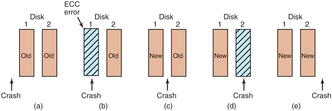
In the absence of CPU crashes, this scheme always works because stable writes always write two valid copies of every block and spontaneous errors are assumed never to occur on both corresponding blocks at the same time. What about in the presence of CPU crashes during stable writes? It depends on precisely when the crash occurs. There are five possibilities, as depicted in Fig. 5-25.
Figure 5-25
Analysis of the influence of crashes on stable writes.
In Fig. 5-25(a), the CPU crash happens before either copy of the block is written. During recovery, neither will be changed and the old value will continue to exist, which is allowed.
In Fig. 5-25(b), the CPU crashes during the write to drive 1, destroying the contents of the block. However, the recovery program detects this error and restores the block on drive 1 from drive 2. Thus, the effect of the crash is wiped out and the old state is fully restored.
In Fig. 5-25(c), the CPU crash happens after drive 1 is written but before drive 2 is written. The point of no return has been passed here: the recovery program copies the block from drive 1 to drive 2. The write succeeds.
Fig. 5-25(d) is like Fig. 5-25(b): during recovery, the good block overwrites the bad block. Again, the final value of both blocks is the new one.
Finally, in Fig. 5-25(e), the recovery program sees that both blocks are the same, so neither is changed and the write succeeds here, too.
Various optimizations and improvements are possible to this scheme. For starters, comparing all the blocks pairwise after a crash is doable, but expensive. A huge improvement is to keep track of which block was being written during a stable write so that only one block has to be checked during recovery. Many computers have a small amount of nonvolatile RAM, which is a special CMOS memory powered by a lithium battery. Such batteries last for years, possibly even the whole life of the computer. Unlike main memory, which is lost after a crash, nonvolatile RAM is not lost after a crash. The time of day is normally kept here (and incremented by a special circuit), which is why computers still know what time it is even after having been unplugged.
Suppose that a few bytes of nonvolatile RAM are available for operating system purposes. The stable write can put the number of the block it is about to update in nonvolatile RAM before starting the write. After successfully completing the stable write, the block number in nonvolatile RAM is overwritten with an invalid block number, for example, Under these conditions, after a crash the recovery program can check the nonvolatile RAM to see if a stable write happened to be in progress during the crash, and if so, which block was being written when the crashed happened. The two copies of the block can then be checked for correctness and consistency.
If nonvolatile RAM is not available, it can be simulated as follows. At the start of a stable write, a fixed disk block on drive 1 is overwritten with the number of the block to be stably written. This block is then read back to verify it. After getting it correct, the corresponding block on drive 2 is written and verified. When the stable write completes correctly, both blocks are overwritten with an invalid block number and verified. Again here, after a crash it is easy to determine whether or not a stable write was in progress during the crash. Of course, this technique requires eight extra disk operations to write a stable block, so it should be used exceedingly sparingly.
One last point is worth making. We assumed that only one spontaneous decay of a good block to a bad block happens per block pair per day. If enough days go by, the other one might go bad, too. Therefore, once a day a complete scan of both disks must be done, repairing any damage. That way, every morning both disks are always identical. Even if both blocks in a pair go bad within a period of a few days, all errors are repaired correctly.
5.4.3 RAID
One technique that now helps improve the reliability of storage systems in general originally became popular as a measure to boost the performance of magnetic disk storage systems. Before SSDs came along, CPU performance had been increasing exponentially for decades, for a long time roughly doubling every 18 months. Not so with disk performance. In the 1970s, average seek times on minicomputer disks were 50 to 100 msec. Today seek times on magnetic disks are still a few msec. In most technical industries (say, automobiles, aviation, or trains), a factor 10 performance improvement in two decades would be major news (imagine 300-MPG cars, flying from Amsterdam to San Francisco in an hour, or taking a train from New York to D.C. in 20 minutes, but in the computer industry it is an embarrassment. Thus, the gap between CPU performance and (hard) disk performance had become much larger over time. Could anything be done to help?
Yes! As we have seen, parallel processing is increasingly being used to speed up computation. It has occurred to various people over the years that parallel I/O might be a good idea, too. In their 1988 paper, Patterson et al. suggested six specific disk organizations that could be used to improve disk performance, reliability, or both (Patterson et al., 1988). These ideas were quickly adopted by industry and have led to a new class of I/O device called a RAID. Patterson et al. defined RAID as Redundant Array of Inexpensive Disks, but industry redefined the I to be ‘‘Independent’’ rather than ‘‘Inexpensive’’ (maybe so they could charge more?). Since a villain was also needed (as in RISC vs. CISC, also due to Patterson), the bad guy here was the SLED (Single Large Expensive Disk).
The fundamental idea behind a RAID is to install a box full of disks next to the computer, typically a large server, replace the disk controller card with a RAID controller, copy the data over to the RAID, and then continue normal operation. In other words, a RAID should look like a SLED to the operating system but have better performance and better reliability. In the past, RAIDs consisted exclusively of hard disks typically connected via SCSI interfaces. Nowadays, manufacturers also support SATA and SSDs as well as disks.
In addition to appearing like a single disk to the software, all RAIDs have the property that the data are distributed over the drives, to allow parallel operation. Several different schemes for doing this were defined by Patterson et al. Nowadays, most manufacturers refer to the seven standard configurations as RAID level 0 through RAID level 6. In addition, there are a few other minor levels that we will not discuss. The term ‘‘level’’ is something of a misnomer since no hierarchy is involved; there are simply seven different organizations possible.
RAID level 0 is illustrated in Fig. 5-26(a). It consists of viewing the virtual single disk simulated by the RAID as being divided up into strips of k sectors each, with sectors 0 to being strip 0, sectors k to strip 1, and so on. For each strip is a sector; for a strip is two sectors, etc. The RAID level 0 organization writes consecutive strips over the drives in round-robin fashion, as depicted in Fig. 5-26(a) for a RAID with four disk drives.
Figure 5-26
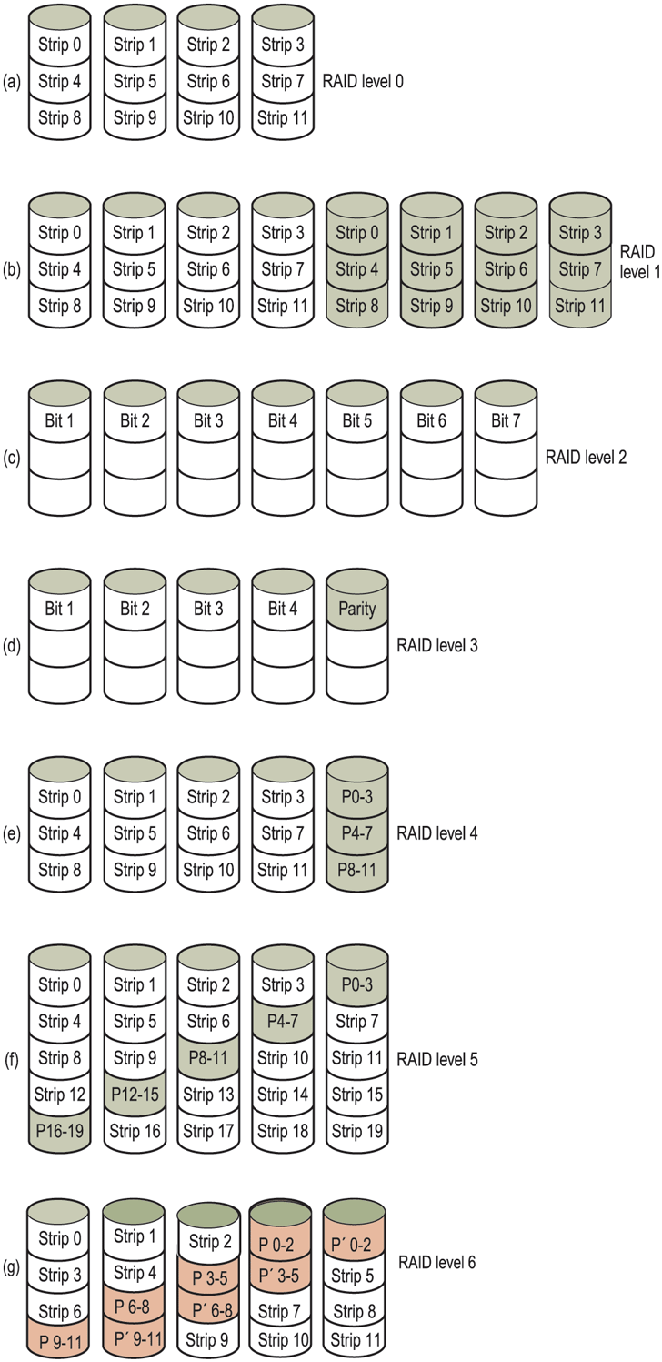
RAID levels 0 through 6. Backup and parity drives are shown shaded.
Distributing data over multiple drives like this is called striping. For example, if the software issues a command to read a data block consisting of four consecutive strips starting at a strip boundary, the RAID controller will break this command up into four separate commands, one for each of the four disks, and have them operate in parallel. Thus, we have parallel I/O without the software knowing about it.
RAID level 0 works best with large requests, the bigger the better. If a request is larger than the number of drives times the strip size, some drives will get multiple requests, so that when they finish the first request they start the second one. It is up to the controller to split the request up and feed the proper commands to the proper disks in the right sequence and then assemble the results in memory correctly. Performance is excellent and the implementation is straightforward.
RAID level 0 works worst with operating systems that habitually ask for data one sector at a time. The results will be correct, but there is no parallelism and hence no performance gain. Another disadvantage of this organization is that the reliability is potentially worse than having a SLED. If a RAID consists of four disks, each with a mean time to failure of 20,000 hours, about once every 5000 hours a drive will fail and all the data will be completely lost. A SLED with a mean time to failure of 20,000 hours would be four times more reliable. Because no redundancy is present in this design, it is not really a true RAID. Remember, the ‘‘R’’ in RAID stands for ‘‘Redundant.’’
The next option, RAID level 1, shown in Fig. 5-26(b), is a true RAID. It duplicates all the disks, so there are four primary disks and four backup disks. On a write, every strip is written twice. On a read, either copy can be used, distributing the load over more drives. Consequently, write performance is no better than for a single drive, but read performance can be up to twice as good. Fault tolerance is excellent: if a drive crashes, the copy is simply used instead. Recovery consists of simply installing a new drive and copying the entire backup drive to it.
Unlike levels 0 and 1, which work with strips of sectors, RAID level 2 works on a word basis, possibly even a byte basis. Imagine splitting each byte of the single virtual disk into a pair of 4-bit nibbles, then adding a Hamming code to each one to form a 7-bit word, of which bits 1, 2, and 4 were parity bits. Further imagine that the seven drives of Fig. 5-26(c) were synchronized in terms of arm position and rotational position. Then it would be possible to write the 7-bit Hamming coded word over the seven drives, one bit per drive.
The Thinking Machines CM-2 computer used this scheme, taking 32-bit data words and adding 6 parity bits to form a 38-bit Hamming word, plus an extra bit for word parity, and spread each word over 39 disk drives. The total throughput was immense, because in one sector time it could write 32 sectors worth of data. Also, losing one drive did not cause problems, because loss of a drive amounted to losing 1 bit in each 39-bit word read, something the Hamming code could handle on the fly.
On the down side, this scheme requires all the drives to be rotationally synchronized, and it only makes sense with a substantial number of drives (even with 32 data drives and 6 parity drives, the overhead is 19%). It also asks a lot of the controller, since it must do a Hamming checksum every bit time.
RAID level 3 is a simplified version of RAID level 2. It is illustrated in Fig. 5-26(d). Here a single parity bit is computed for each data word and written to a parity drive. As in RAID level 2, the drives must be exactly synchronized, since individual data words are spread over multiple drives.
At first thought, it might appear that a single parity bit gives only error detection, not error correction. For the case of random undetected errors, this is true.
However, for the case of a drive crashing, it provides full 1-bit error correction since the position of the bad bit is known. In the event that a drive crashes, the controller just pretends that all its bits are 0s. If a word has a parity error, the bit from the dead drive must have been a 1, so it is corrected. Although both RAID levels 2 and 3 offer very high data rates, the number of separate I/O requests per second they can handle is no better than for a single drive.
RAID levels 4 and 5 work with strips again, not individual words with parity, and do not require synchronized drives. RAID level 4 [see Fig. 5-26(e)] is like RAID level 0, with a strip-for-strip parity written onto an extra drive. For example, if each strip is k bytes long, all the strips are EXCLUSIVE ORed together, resulting in a parity strip k bytes long. If a drive crashes, the lost bytes can be recomputed from the parity drive by reading the entire set of drives.
This design protects against the loss of a drive but performs poorly for small updates. If one sector is changed, it is necessary to read all the drives in order to recalculate the parity, which must then be rewritten. Alternatively, it can read the old user data and the old parity data and recompute the new parity from them. Even with this optimization, a small update requires two reads and two writes.
As a consequence of the heavy load on the parity drive, it may become a bottleneck. This bottleneck is eliminated in RAID level 5 by distributing the parity bits uniformly over all the drives, round-robin fashion, as shown in Fig. 5-26(f). However, in the event of a drive crash, reconstructing the contents of the failed drive is a complex process.
Raid level 6 is similar to RAID level 5, except that an additional parity block is used. In other words, the data are striped across the disks with two parity blocks instead of one. As a result, writes are bit more expensive because of the parity calculations, but reads incur no performance penalty. It does offer more reliability (imagine what happens if RAID level 5 encounters a bad block just when it is rebuilding its array).
Compared to magnetic disks, SSDs offer much better performance and much higher reliability. Do we still need RAID? The answer may still be yes. After all, a RAID of multiple SSDs can offer even better performance and reliability than a single SSD. For instance, RAID level 0 with two SSDs provides sequential read and write performance that is roughly double that of a single SSD. If sequential read/write performance is important in your storage stack, this may be a winner. Of course, RAID level 0 does not help and even diminishes reliability, but maybe that is less bad for SSDs than for magnetic disks that fail more easily. Moreover, for reliability we can opt for higher RAID levels, such as RAID level 1. RAID level 1 may improve the read performance (since even if one SSD is busy, the other is still available), but not write performance as all data must be stored twice and errors verified. Also, since you can only use half of your storage capacity, RAID level 1 is expensive—especially since compared to magnetic disks, SSDs are not cheap.
Although RAID levels 5 and 6 are also used with SSD, with the benefit of some performance gains and increased reliability, they do have drawbacks. In particular, they are ‘‘write-heavy’’ and require a fair number of additional writes due to the parity blocks. Unfortunately, writes are not just relatively expensive, they also increase the SSD’s wear.