4.3 File-System Implementation
Now it is time to turn from the user’s view of the file system to the implementor’s view. Users are concerned with how files are named, what operations are allowed on them, what the directory tree looks like, and similar interface issues. Implementers are interested in how files and directories are stored, how disk space is managed, and how to make everything work efficiently and reliably. In the following sections, we will examine a number of these areas to see what the issues and trade-offs are.
4.3.1 File-System Layout
File systems are stored on disks. Most disks can be divided up into one or more partitions, with independent file systems on each partition. The layout depends on whether you have an old computer with a BIOS and a master boot record, or a modern UEFI-based system.
Old School: The Master Boot Record
On older systems, sector 0 of the disk is called the MBR (Master Boot Record) and is used to boot the computer. The end of the MBR contains the partition table. This table gives the starting and ending addresses of each partition. One of the partitions in the table is marked as active. When the computer is booted, the BIOS reads in and executes the MBR. The first thing the MBR program does is locate the active partition, read in its first block, which is called the boot block, and execute it. The program in the boot block loads the operating system contained in that partition. For uniformity, every partition starts with a boot block, even if it does not contain a bootable operating system. Besides, it might contain one in the future.
Other than starting with a boot block, the layout of a disk partition varies a lot from file system to file system. Often the file system will contain some of the items shown in Fig. 4-10. The first one is the superblock. It contains all the key parameters about the file system and is read into memory when the computer is booted or the file system is first touched. Typical information in the superblock includes a magic number to identify the file-system type, the number of blocks in the file system, and other key administrative information.
Figure 4-10
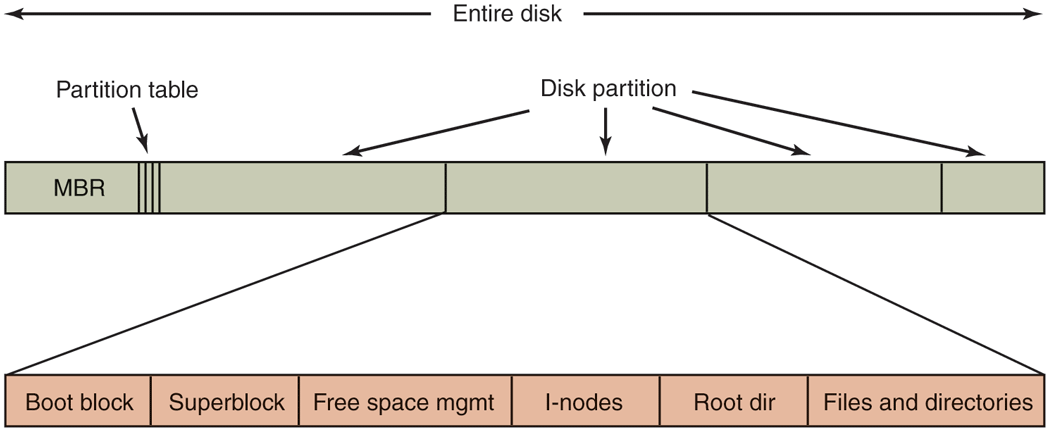
A possible file-system layout.
Next might come information about free blocks in the file system, for example in the form of a bitmap or a list of pointers. This might be followed by the i-nodes, an array of data structures, one per file, telling all about the file. After that might come the root directory, which contains the top of the file-system tree. Finally, the remainder of the disk contains all the other directories and files.
New School: Unified Extensible Firmware Interface
Unfortunately, booting in the way described above is slow, architecture-dependent, and limited to smaller disks (up to 2 TB) and Intel therefore proposed the UEFI (Unified Extensible Firmware Interface) as a replacement. is now the most popular way to boot personal computer systems. It fixes many of the problems of the old-style BIOS and MBR: fast booting, different architectures, and disk sizes up to 8 ZiB. It is also quite complex.
Rather than relying on a Master Boot Record residing in sector 0 of the boot device, UEFI looks for the location of the partition table in the second block of the device. It reserves the first block as a special marker for software that expects an MBR here. The marker essentially says: No MBR here!
The GPT (GUID Partition Table), meanwhile, contains information about the location of the various partitions on the disk. GUID stands for globally unique identifiers. As shown in Fig. 4-11, UEFI keeps a backup of the GPT in the last block. A GPT contains the start and end of each partition. Once the GPT is found, the firmware has enough functionality to read file systems of specific types. According to the UEFI standard the firmware should support at least FAT file system types. One such file system is placed in a special disk partition, known as the EFI system partition (ESP). Rather than a single magic boot sector, the boot process can now use a proper file system containing programs, configuration files, and anything else that may be useful during boot. Moreover, UEFI expects the firmware to be able to execute programs in a specific format, called PE (Portable Executable). In other words, the firmware under UEFI looks like a small operating system itself with an understanding of disk partitions, file systems, executables, etc.
Figure 4-11
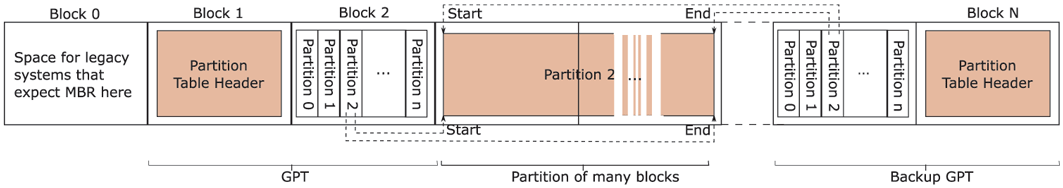
Layout for UEFI with partition table.
4.3.2 Implementing Files
Probably the most important issue in implementing file storage is keeping track of which disk blocks go with which file. Various methods are used in different operating systems. In this section, we will examine a few of them.
Contiguous Allocation
The simplest allocation scheme is to store each file as a contiguous run of disk blocks. Thus on a disk with 1-KB blocks, a 50-KB file would be allocated 50 consecutive blocks. With 2-KB blocks, it would be allocated 25 consecutive blocks.
We see an example of contiguous storage allocation in Fig. 4-12(a). Here the first 40 disk blocks are shown, starting with block 0 on the left. Initially, the disk was empty. Then a file A, of length four blocks, was written to disk starting at the beginning (block 0). After that a six-block file, B, was written starting right after the end of file A.
Figure 4-12
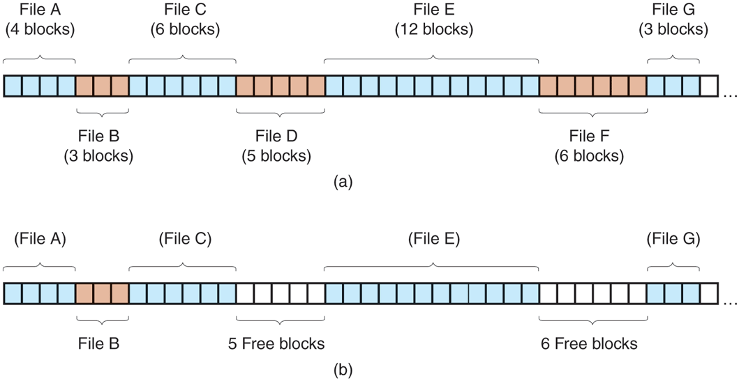
(a) Contiguous allocation of disk space for seven files. (b) The state of the disk after files D and F have been removed.
Note that each file begins at the start of a new block, so that if file A was really 3½ blocks, some space is wasted at the end of the last block. In the figure, a total of seven files are shown, each one starting at the block following the end of the previous one. Shading is used just to make it easier to tell the files apart. It has no actual significance in terms of storage.
Contiguous disk-space allocation has two significant advantages. First, it is simple to implement because keeping track of where a file’s blocks are is reduced to remembering two numbers: the disk address of the first block and the number of blocks in the file. Given the number of the first block, the number of any other block can be found by a simple addition.
Second, the read performance is excellent even on a magnetic disk because the entire file can be read from the disk in a single operation. Only one seek is needed (to the first block). After that, no more seeks or rotational delays are needed, so data come in at the full bandwidth of the disk. Thus contiguous allocation is simple to implement and has high performance. We will talk about sequential versus random accesses on SSDs later.
Unfortunately, contiguous allocation also has a very serious drawback: over the course of time, the disk becomes fragmented. To see how this comes about, examine Fig. 4-12(b). Here two files, D and F, have been removed. When a file is removed, its blocks are naturally freed, leaving a run of free blocks on the disk. The disk is not compacted on the spot to squeeze out the hole, since that would involve copying all the blocks following the hole, potentially millions of blocks, which would take hours or even days with large disks. As a result, the disk ultimately consists of files and holes, as illustrated in the figure.
Initially, this fragmentation is not a problem, since each new file can be written at the end of disk, following the previous one. However, eventually the disk will fill up and it will become necessary to either compact the disk, which is prohibitively expensive, or to reuse the free space in the holes. Reusing the space requires maintaining a list of holes, which is doable. However, when a new file is to be created, it is necessary to know its final size in order to choose a hole that is big enough.
Imagine the consequences of such a design. The user starts a recording application in order to create a video. The first thing the program asks is how many bytes the final video will be. The question must be answered or the program will not continue. If the number given ultimately proves too small, the program has to terminate prematurely because the disk hole is full and there is no place to put the rest of the file. If the user tries to avoid this problem by giving an unrealistically large number as the final size, say, 100 GB, the editor may be unable to find such a large hole and announce that the file cannot be created. Of course, the user would be free to start the program again, say 50 GB this time, and so on until a suitable hole was located. Still, this scheme is not likely to lead to happy users.
Linked-List Allocation
The second method for storing files is to keep each one as a linked list of disk blocks, as shown in Fig. 4-13. The first part of each block is used as a pointer to the next one. The rest of the block is for data.
Figure 4-13
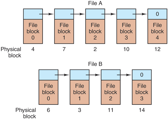
Storing a file as a linked list of disk blocks.
Unlike contiguous allocation, every disk block can be used in this method. No space is lost to disk fragmentation (except for internal fragmentation in the last block). Also, it is sufficient for the directory entry to merely store the disk address of the first block. The rest can be found starting there.
On the other hand, although reading a file sequentially is straightforward, random access is extremely slow. To get to block n, the operating system has to start at the beginning and read the blocks prior to it, one at a time. Clearly, doing so many reads will be painfully slow.
Also, the amount of data storage in a block is no longer a power of two because the pointer takes up a few bytes. While not fatal, having a peculiar size is less efficient because many programs read and write in blocks whose size is a power of two. With the first few bytes of each block occupied by a pointer to the next block, reads of the full block size require acquiring and concatenating information from two disk blocks, which generates extra overhead due to the copying.
Linked-List Allocation Using a Table in Memory
Both disadvantages of the linked-list allocation can be eliminated by taking the pointer word from each disk block and putting it in a table in memory. Figure 4-14 shows what the table looks like for the example of Fig. 4-13. In both figures, we have two files. File A uses disk blocks 4, 7, 2, 10, and 12, in that order, and file B uses disk blocks 6, 3, 11, and 14, in that order. Using the table of Fig. 4-14, we can start with block 4 and follow the chain all the way to the end. The same can be done starting with block 6. Both chains are terminated with a special marker (e.g., ) that is not a valid block number. Such a table in main memory is called a FAT(File Allocation Table).
Figure 4-14
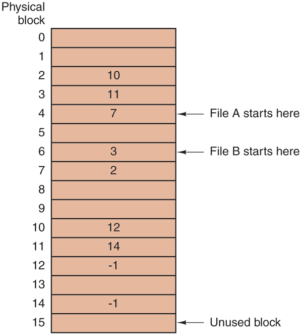
Linked-list allocation using a file-allocation table in main memory.
Using this organization, the entire block is available for data. Furthermore, random access is much easier. Although the chain must still be followed to find a given offset within the file, the chain is entirely in memory, so it can be followed without making any disk references. Like the previous method, it is sufficient for the directory entry to keep a single integer (the starting block number) and still be able to locate all the blocks, no matter how large the file is.
The primary disadvantage of this method is that the entire table must be in memory all the time to make it work. With a 1-TB disk and a 1-KB block size, the table needs 1 billion entries, one for each of the 1 billion disk blocks. Each entry has to be a minimum of 3 bytes. For speed in lookup, they should be 4 bytes. Thus the table will take up 3 GB or 2.4 GB of main memory all the time, depending on whether the system is optimized for space or time. Not wildly practical. Clearly the FAT idea does not scale well to large disks. Nevertheless, it was the original MSDOS file system and is still fully supported by all versions of Windows though (and UEFI). Versions of the FAT file system are still commonly used on the SD cards used in digital cameras, electronic picture frames, music players, and other portable electronic devices, as well as in other embedded applications.
I-nodes
Our last method for keeping track of which blocks belong to which file is to associate with each file a data structure called an i-node (index-node), which lists the attributes and disk addresses of the file’s blocks. A simple example is depicted in Fig. 4-15. Given the i-node, it is then possible to find all the blocks of the file. The big advantage of this scheme over linked files using an in-memory table is that the i-node needs to be in memory only when the corresponding file is open. If each i-node occupies n bytes and a maximum of k files may be open at once, the total memory occupied by the array holding the i-nodes for the open files is only kn bytes. Only this much space need be reserved in advance.
Figure 4-15
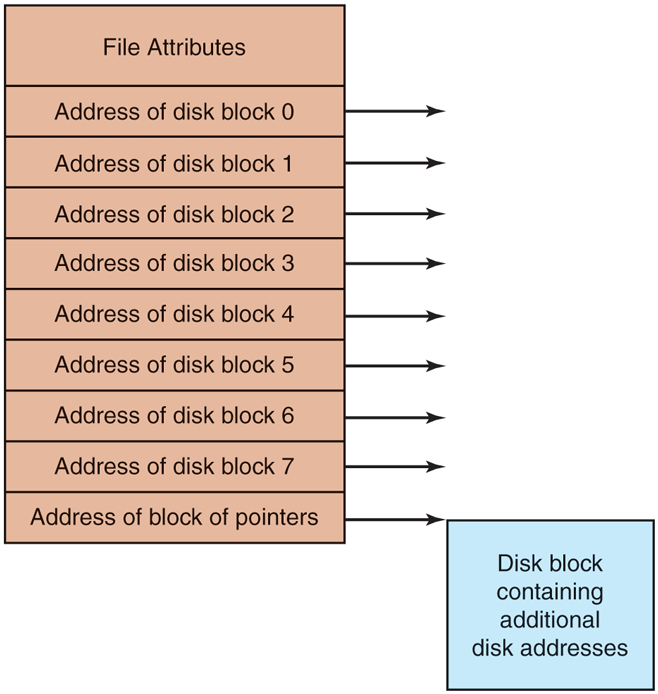
An example i-node.
This array is usually far smaller than the space occupied by the file table described in the previous section. The reason is simple. The table for holding the linked list of all disk blocks is proportional in size to the disk itself. If the disk has n blocks, the table needs n entries. As disks grow larger, this table grows linearly with them. In contrast, the i-node scheme requires an array in memory whose size is proportional to the maximum number of files that may be open at once. It does not matter if the disk is 500 GB, 500 TB, or 500 PB.
One problem with i-nodes is that if each one has room for a fixed number of disk addresses, what happens when a file grows beyond this limit? One solution is to reserve the last disk address not for a data block, but instead for the address of a block containing more disk-block addresses, as shown in Fig. 4-15. Even more advanced would be two or more such blocks containing disk addresses or even disk blocks pointing to other disk blocks full of addresses. We will come back to inodes when studying UNIX in Chapter 10. Similarly, the Windows NTFS file system uses a similar idea, only with bigger i-nodes that can also contain small files.
4.3.3 Implementing Directories
Before a file can be read, it must be opened. When a file is opened, the operating system uses the path name supplied by the user to locate the directory entry on the disk. The directory entry provides the information needed to find the disk blocks. Depending on the system, this information may be the disk address of the entire file (with contiguous allocation), the number of the first block (both linked-list schemes), or the number of the i-node. In all cases, the main function of the directory system is to map the ASCII name of the file onto the information needed to locate the data.
A closely related issue is where the attributes should be stored. Every file system maintains various file attributes, such as each file’s owner and creation time, and they must be stored somewhere. One obvious possibility is to store them directly in the directory entry. Some systems do precisely that. This option is shown in Fig. 4-16(a). In this simple design, a directory consists of a list of fixedsize entries, one per file, containing a (fixed-length) file name, a structure of the file attributes, and one or more disk addresses (up to some maximum) telling where the disk blocks are.
Figure 4-16
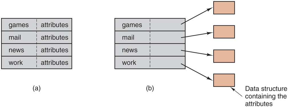
(a) A simple directory containing fixed-size entries with the disk addresses and attributes in the directory entry. (b) A directory in which each entry justrefers to an i-node.
For systems that use i-nodes, another possibility for storing the attributes is in the i-nodes, rather than in the directory entries. In that case, the directory entry can be shorter: just a file name and an i-node number. This approach is illustrated in Fig. 4-16(b). As we shall see later, this method has some advantages over putting them in the directory entry.
So far we have made the implicit assumption that files have short, fixed-length names. In MS-DOS files have a 1–8 character base name and an optional extension of 1–3 characters. In UNIX Version 7, file names were 1–14 characters, including any extensions. However, nearly all modern operating systems support longer, variable-length file names. How can these be implemented?
The simplest approach is to set a limit on file-name length, typically 255 characters, and then use one of the designs of Fig. 4-16 with 255 characters reserved for each file name. This approach is simple, but wastes a great deal of directory space, since few files have such long names. For efficiency reasons, a different structure is desirable.
One alternative is to give up the idea that all directory entries are the same size. With this method, each directory entry contains a fixed portion, typically starting with the length of the entry, and then followed by data with a fixed format, usually including the owner, creation time, protection information, and other attributes. This fixed-length header is followed by the actual file name, however long it may be, as shown in Fig. 4-17(a) in big-endian format (as used by some CPUs). In this example we have three files, project-budget, personnel, and foo. Each file name is terminated by a special character (usually 0), which is represented in the figure by a box with a cross in it. To allow each directory entry to begin on a word boundary, each file name is filled out to an integral number of words, shown by shaded boxes in the figure.
Figure 4-17
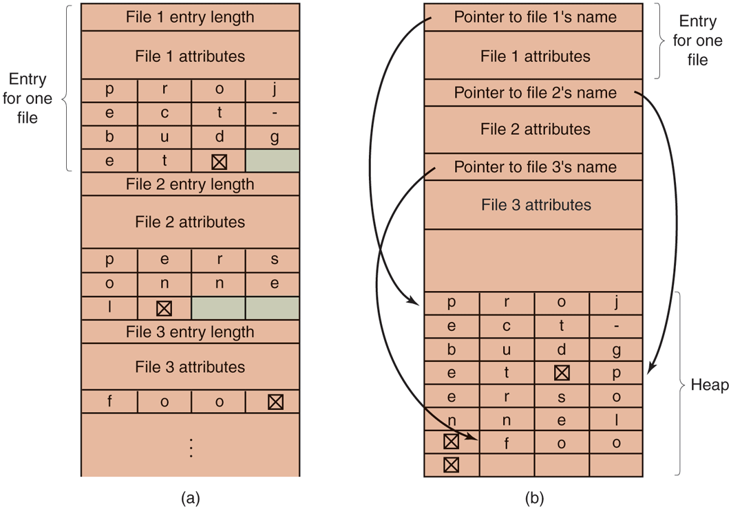
Two ways of handling long file names in a directory. (a) In-line. (b) In a heap.
A disadvantage of this method is that when a file is removed, a variable-sized gap is introduced into the directory into which the next file to be entered may not fit. This problem is essentially the same one we saw with contiguous disk files, only now compacting the directory is feasible because it is entirely in memory. Another problem is that a single directory entry may span multiple pages, so a page fault may occur while reading a file name.
Another way to handle variable-length names is to make the directory entries themselves all fixed length and keep the file names together in a heap at the end of the directory, as shown in Fig. 4-17(b). This method has the advantage that when an entry is removed, the next file entered will always fit there. Of course, the heap must be managed and page faults can still occur while processing file names. One very minor win here is that there is no longer any real need for file names to begin at word boundaries, so no filler characters are needed after file names in Fig. 4-17(b) as they are in Fig. 4-17(a).
In all of the designs so far, directories are searched linearly from beginning to end when a file name has to be looked up. For extremely long directories, linear searching can be slow. One way to speed up the search is to use a hash table in each directory. Call the size of the table n. To enter a file name, the name is hashed onto a value between 0 and for example, by dividing it by n and taking the remainder. Alternatively, the words comprising the file name can be added up and this quantity divided by n, or something similar.
Either way, the table entry corresponding to the hash code is inspected. If it is unused, a pointer is placed there to the file entry. File entries follow the hash table. If that slot is already in use, a linked list is constructed, headed at the table entry and threading through all entries with the same hash value.
Looking up a file follows the same procedure. The file name is hashed to select a hash-table entry. All the entries on the chain headed at that slot are checked to see if the file name is present. If the name is not on the chain, the file is not present in the directory.
Using a hash table has the advantage of much faster lookup, but the disadvantage of a much more complex administration. It is only really a serious candidate in systems where it is expected that directories will routinely contain hundreds or thousands of files.
A different way to speed up searching large directories is to cache the results of searches. Before starting a search, a check is first made to see if the file name is in the cache. If so, it can be located immediately. Of course, caching only works if a relatively small number of files comprise the majority of the lookups.
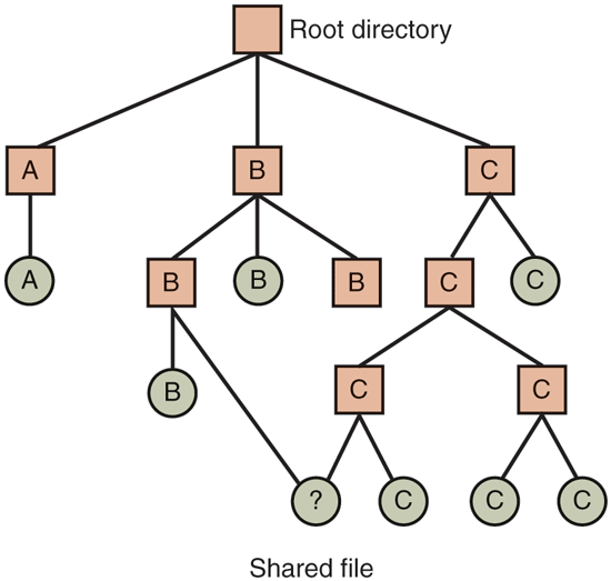
4.3.4 Shared Files
When several users are working together on a project, they often need to share files. As a result, it is often convenient for a shared file to appear simultaneously in different directories belonging to different users. Figure 4-18 shows the file system of Fig. 4-8 again, only with one of C’s files now present in one of B’s directories as well. The connection between B’s directory and the shared file is called a link. The file system itself is now a DAG (Directed Acyclic Graph), rather than a tree. Having the file system be a DAG complicates maintenance, but such is life.
Figure 4-18
File system containing a shared file.
Sharing files is convenient, but it also introduces some problems. To start with, if directories really do contain disk addresses, then a copy of the disk addresses will have to be made in B’s directory when the file is linked. If either B or C subsequently appends to the file, the new blocks will be listed only in the directory of the user doing the append. The changes will not be visible to the other user, thus defeating the purpose of sharing.
This problem can be solved in two ways. In the first solution, disk blocks are not listed in directories, but in a little data structure associated with the file itself. The directories would then just have pointers to the little data structure. This is the approach used in UNIX (where the little data structure is the i-node).
In the second solution, B links to one of C’s files by having the system create a new file, of type LINK, and entering that file in B’s directory. The new file contains just the path name of the file to which it is linked. When B reads from the linked file, the operating system sees that the file being read from is of type LINK, looks up the name of the file, and reads that file. This approach is called symbolic linking, to contrast it with traditional (hard) linking, as discussed earlier.
Each of these methods has its drawbacks. In the first method, at the moment that B links to the shared file, the i-node records the file’s owner as C. Creating a link does not change the ownership (see Fig. 4-19), but it does increase the link count in the i-node, so the system knows how many directory entries currently point to the file.
Figure 4-19
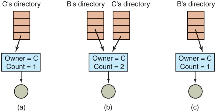
(a) Situation prior to linking. (b) After the link is created. (c) After the original owner removes the file.
If C subsequently tries to remove the file, the system is faced with a problem. If it removes the file and clears the i-node, B will have a directory entry pointing to an invalid i-node. If the i-node is later reassigned to another file, B’s link will point to the wrong file. The system can see from the count in the i-node that the file is still in use, but there is no easy way for it to find all the directory entries for the file, in order to erase them. Pointers to the directories cannot be stored in the i-node because there can be an unlimited number of directories.
The only thing to do is remove C’s directory entry, but leave the i-node intact, with count set to 1, as shown in Fig. 4-19(c). We now have a situation in which B is the only user having a directory entry for a file owned by C. If the system does accounting or has quotas, C will continue to be billed for the file until B decides to remove it, if ever, at which time the count goes to 0 and the file is deleted.
With symbolic links this problem does not arise because only the true owner has a pointer to the i-node. Users who have linked to the file just have path names, not i-node pointers. When the owner removes the file, it is destroyed. Subsequent attempts to use the file via a symbolic link will fail when the system is unable to locate the file. Removing a symbolic link does not affect the file at all.
The problem with symbolic links is the extra overhead required. The file containing the path must be read, then the path must be parsed and followed, component by component, until the i-node is reached. All of this activity may require a considerable number of extra disk accesses. Furthermore, an extra i-node is needed for each symbolic link, as is an extra disk block to store the path, although if the path name is short, the system could store it in the i-node itself, as a kind of optimization. Symbolic links have the advantage that they can be used to link to files on machines anywhere in the world, by simply providing the network address of the machine where the file resides in addition to its path on that machine.
There is also another problem introduced by links, symbolic or otherwise. When links are allowed, files can have two or more paths. Programs that start at a given directory and find all the files in that directory and its subdirectories will locate a linked file multiple times. For example, a program that dumps all the files in a directory and its subdirectories onto a backup drive may make multiple copies of a linked file. Furthermore, if the backup drive is then read into another machine, unless the dump program is clever, the linked file may be copied twice onto the disk, instead of being linked.
4.3.5 Log-Structured File Systems
Changes in technology are putting pressure on current file systems. Let us consider computers with (magnetic) hard disks. In the next section, we will look at SSDs. In systems with hard disks, the CPUs keep getting faster, the disks are becoming much bigger and cheaper (but not much faster), and memories are growing exponentially in size. The one parameter that is not improving by leaps and bounds is disk seek time.
The combination of these factors led to a performance bottleneck in file systems. Research done at Berkeley attempted to alleviate this problem by designing a completely new kind of file system, LFS (the Log-structured File System). In this section, we will briefly describe how LFS works. For a more complete treatment, see the original paper on LFS (Rosenblum and Ousterhout, 1991).
The idea that drove the LFS design is that as CPUs get faster and RAM memories get larger, disk caches are also increasing rapidly. Consequently, it is now possible to satisfy a very substantial fraction of all read requests directly from the file-system cache, with no disk access needed. It follows from this observation that in the future, most disk accesses will be writes, so the read-ahead mechanism used in some file systems to fetch blocks before they are needed no longer gains much performance.
To make matters worse, in most file systems, writes are done in very small chunks. Small writes are highly inefficient, since a disk write is often preceded by a 10-msec seek and a 4-msec rotational delay. With these parameters, disk efficiency drops to a fraction of 1%.
To see where all the small writes come from, consider creating a new file on a UNIX system. To write this file, the i-node for the directory, the directory block, the i-node for the file, and the file itself must all be written. While these writes can be delayed, doing so exposes the file system to serious consistency problems if a crash occurs before the writes are done. For this reason, the i-node writes are generally done immediately.
From this reasoning, the LFS designers decided to reimplement the UNIX file system in such a way as to achieve the full bandwidth of the disk, even in the face of a workload consisting in large part of small random writes. The basic idea is to structure the entire disk as a great big log.
Periodically, and when there is a special need for it, all the pending writes being buffered in memory are collected into a single segment and written to the disk as a single contiguous segment at the end of the log. A single segment may thus contain i-nodes, directory blocks, and data blocks, all mixed together. At the start of each segment is a segment summary, telling what can be found in the segment. If the average segment can be made to be about 1 MB, almost the full bandwidth of the disk can be utilized.
In this design, i-nodes still exist and even have the same structure as in UNIX, but they are now scattered all over the log, instead of being at a fixed position on the disk. Nevertheless, when an i-node is located, locating the blocks is done in the usual way. Of course, finding an i-node is now much harder, since its address cannot simply be calculated from its i-number, as in UNIX. To make it possible to find i-nodes, an i-node map, indexed by i-number, is maintained. Entry i in this map points to i-node i on the disk. The map is kept on disk, but it is also cached, so the most heavily used parts will be in memory most of the time.
To summarize what we have said so far, all writes are initially buffered in memory, and periodically all the buffered writes are written to the disk in a single segment, at the end of the log. Opening a file now consists of using the map to locate the i-node for the file. Once the i-node has been located, the addresses of the blocks can be found from it. All of the blocks will themselves be in segments, somewhere in the log.
If disks were infinitely large, the above description would be the entire story. However, real disks are finite, so eventually the log will occupy the entire disk, at which time no new segments can be written to the log. Fortunately, many existing segments may have blocks that are no longer needed. For example, if a file is overwritten, its i-node will now point to the new blocks, but the old ones will still be occupying space in previously written segments.
To deal with this problem, LFS has a cleaner thread that spends its time scanning the log circularly to compact it. It starts out by reading the summary of the first segment in the log to see which i-nodes and files are there. It then checks the current i-node map to see if the i-nodes are still current and file blocks are still in use. If not, that information is discarded. The i-nodes and blocks that are still in use go into memory to be written out in the next segment. The original segment is then marked as free, so that the log can use it for new data. In this manner, the cleaner moves along the log, removing old segments from the back and putting any live data into memory for rewriting in the next segment. Consequently, the disk is a big circular buffer, with the writer thread adding new segments to the front and the cleaner thread removing old ones from the back.
The bookkeeping here is nontrivial, since when a file block is written back to a new segment, the i-node of the file (somewhere in the log) must be located, updated, and put into memory to be written out in the next segment. The i-node map must then be updated to point to the new copy. Nevertheless, it is possible to do the administration, and the performance results show that all this complexity is worthwhile. Measurements given in the papers cited above show that LFS outperforms UNIX by an order of magnitude on small writes, while having a performance that is as good as or better than UNIX for reads and large writes.
4.3.6 Journaling File Systems
Log-structured file systems are an interesting idea in general and one of the ideas inherent in them, robustness in the face of failure, can also be applied to more conventional file systems. The basic idea here is to keep a log of what the file system is going to do before it does it, so that if the system crashes before it can do its planned work, upon rebooting the system can look in the log to see what was going on at the time of the crash and finish the job. Such file systems, called journaling file systems, are very popular. Microsoft’s NTFS file system and the Linux ext4 and ReiserFS file systems all use journaling. MacOS offers journaling file systems as an option. Journaling is the default and it is widely used. Below we will give a brief introduction to this topic.
To see the nature of the problem, consider a simple garden-variety operation that happens all the time: removing a file. This operation (in UNIX) requires three steps:
Remove the file from its directory.
Release the i-node to the pool of free i-nodes.
Return all the disk blocks to the pool of free disk blocks.
In Windows, analogous steps are required. In the absence of system crashes, the order in which these steps are taken does not matter; in the presence of crashes, it does. Suppose that the first step is completed and then the system crashes. The i-node and file blocks will not be accessible from any file, but will also not be available for reassignment; they are just off in limbo somewhere, decreasing the available resources. If the crash occurs after the second step, only the blocks are lost.
If the order of operations is changed and the i-node is released first, then after rebooting, the i-node may be reassigned, but the old directory entry will continue to point to it, hence to the wrong file. If the blocks are released first, then a crash before the i-node is cleared will mean that a valid directory entry points to an i-node listing blocks now in the free storage pool and which are likely to be reused shortly, leading to two or more files randomly sharing the same blocks. None of these outcomes are good.
What the journaling file system does is first write a log entry listing the three actions to be completed. The log entry is then written to disk (and for good measure, possibly read back from the disk to verify that it was, in fact, written correctly). Only after the log entry has been written, do the various operations begin. After the operations complete successfully, the log entry is erased. If the system now crashes, upon recovery the file system can check the log to see if any operations were pending. If so, all of them can be rerun (multiple times in the event of repeated crashes) until the file is correctly removed.
To make journaling work, the logged operations must be idempotent, which means they can be repeated as often as needed without harm. Operations such as ‘‘Update the bitmap to mark i-node k or block n as free’’ can be repeated until the cows come home with no danger. Similarly, searching a directory and removing any entry called foobar is also idempotent. On the other hand, adding the newly freed blocks from i-node k to the end of the free list is not idempotent since they may already be there. The more-expensive operation ‘‘Search the list of free blocks and add block n to it if it is not already present’’ is idempotent. Journaling file systems have to arrange their data structures and loggable operations so they all are idempotent. Under these conditions, crash recovery can be made fast and secure.
For added reliability, a file system can introduce the database concept of an atomic transaction. When this concept is used, a group of actions can be bracketed by the begin transaction and end transaction operations. The file system then knows it must complete either all the bracketed operations or none of them, but not any other combinations.
NTFS has an extensive journaling system and its structure is rarely corrupted by system crashes. It has been in development since its first release with Windows NT in 1993. The first Linux file system to do journaling was ReiserFS, but its popularity was impeded by the fact that it was incompatible with the then-standard ext2 file system. In contrast, ext3 which was a less ambitious project than ReiserFS, also does journaling while maintaining compatibility with the previous ext2 system. Its successor, ext4 was similarly developed initially as a series of backward-compatible extensions to ext3.
4.3.7 Flash-based File Systems
SSDs uses flash memory and operates quite differently from hard disk drives. Generally, NAND-based flash is used (rather than NOR-based flash) in SSDs. Much of the difference is related to the physics that underpins the storage, which, however fascinating, is beyond the scope of this chapter. Irrespective of the flash technology, here are important differences between hard disks and flash storage. There are no moving parts in flash storage and the problems of seek times and rotational delays that we mentioned in the previous section do not exist. This means that the access time (latency) is much better—on the order of several tens of microseconds instead of milliseconds. It also means that on SSDs there is not much of a gap in performance between random and sequential reads. As we shall see, random writes are still quite a bit more expensive—especially small ones.
Indeed, unlike magnetic disks, flash technology has asymmetric read and write performance: reads are much faster than writes. For instance, where a read takes a few tens of microseconds, a write can take hundreds. First, writes are slow because of how the flash cells that implement the bits are programmed—this is physics and not something we want to get into here. A second, and more impactful reason is that you can only write a unit of data after you have erased a suitable area on the device. In fact, flash memory distinguishes between a unit of I/O (often 4 KB), and a unit of erase (often 64-256 units of I/O, so up to several MB). Sadly, the industry takes great pleasure in confusing people and refers to a unit of I/O as a page and to the unit of erase as a block, except for those publications that refer to the unit of I/O as a block or even a sector and the unit of erase as a chunk. Of course, the meaning of a page is also quite different from that of a memory page in the previous chapter and the meaning of a block does not match that of a disk block either. To avoid confusion, we will use the terms flash page and flash block for the unit of I/O and the unit of erase, respectively.
To write a flash page, the SSD must first erase a flash block—an expensive operation taking hundreds of microseconds. Fortunately, after it has erased the block, there are many free flash pages in that space and the SSD can now write the flash pages in the flash block in order. In other words, it first writes flash page 0 in the block, then 1, then 2, etc. It cannot write flash page 0, followed by 2, and then 1. Also, the SSD cannot really overwrite a flash page that was written earlier. It first has to erase the entire flash block again (not just the page). Indeed, if you really wanted to overwrite some data in a file in-place, the SSD would need to save the other flash pages in the block somewhere else, erase the block in its entirety, and then rewrite the pages one by one—not a cheap operation at all! Instead, modifying data on an SSD simply makes the old flash page invalid and then rewrites the new content in another block. If there are no blocks with free pages available, this would require erasing a block first.
You do not want to keep writing the same flash pages all the time anyway, as flash memory suffers from wear. Repeatedly writing and erasing takes its toll and at some point the flash cells that hold the bits can no longer be used. A program/erase (P/E) cycle consists of erasing a cell and writing new content in it. Typical flash memory cells have a maximum endurance of a few thousand to a few hundred thousand P/E cycles before they kick the bucket. In other words, it is important to spread the wear across the flash memory cells as much as possible.
The device component that is responsible for handling such wear-leveling is known as the FTL (Flash Translation Layer). It has many other responsibilities also and it is sometimes referred to as the drive’s secret sauce. The secret sauce typically runs on a simple processor with access to fast memory. It is shown on the left in Fig. 4-20. The data are stored in the flash packages (FPs) on the right. Each flash package consists of multiple dies and each die in turn contains a number of so-called planes: collections of flash blocks containing flash pages.
Figure 4-20
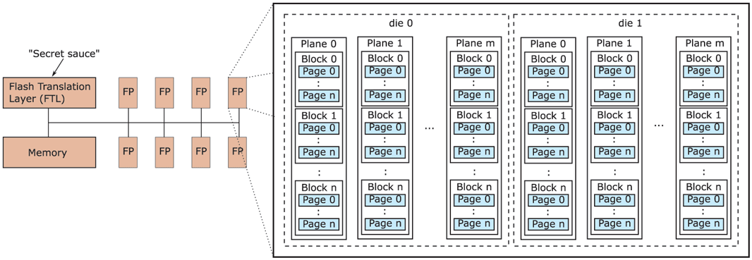
Components inside a typical flash SSD.
To access a specific flash page on the SSD, we need to address the corresponding die on the appropriate flash package, and on that die the right plane, block and page—a rather complicated, hierarchical address! Unfortunately, this is not how file systems work at all. The file system simply requests to read a disk block at a linear, logical disk address. How does the SSD translate between these logical addresses and the complex physical addresses on the device? Here is a hint: the Flash Translation Layer was not given its name for nothing.
Much like the paging mechanism in virtual memory, the FTL uses translation tables to indicate that logical block 54321 is really at die 0 of flash package 1, in plane 2 and block 5. Such translation tables are handy also for wear leveling, since the device is free to move a page to a different block (for instance, because it needs to be updated), as long as it adjusts the mapping in the translation table.
The FTL also takes care of managing blocks and pages that are no longer needed. Suppose that after deleting or moving data a few times, a flash block contains several invalid flash pages. Since only some of the pages are now valid, the device can free up space by copying the remaining valid pages to a block which still has free pages available and then erasing the original block. This is known as garbage collection. In reality, things are much more complicated. For instance, when do we do garbage collection? If we do it constantly and as early as possible, it may interfere with the user’s I/O requests. If we do it too late, we may run out of free blocks. A reasonable compromise is to do it during idle periods, when the SSD is not busy otherwise.
In addition, the garbage collector needs to select both a victim block (the flash block to clean) and a target block (to which to write the live data still in the victim block). Should it simply pick these blocks in a random or round-robin fashion, or try to make a more informed decision? For instance, for the victim block, should it select the flash block with the least amount of valid data, or perhaps avoid the flash blocks that have a lot of wear already, or the blocks that contain a lot of ‘‘hot’’ data (i.e., data that is likely to be written again in the near future anyway)? Likewise, for the target block, should it pick based on the amount of available space, or the amount of accumulated wear on the flash block? Moreover, should it try to group hot and cold data to ensure that cold flash pages can mostly stay in the same block with no need for moving them around, while hot pages will perhaps be updated together close in time, so we can collect the updates in memory and then write them out to a new flash block in one blast? The answer is: yes. And if you’re wondering which strategy is best, the answer is: it depends. Modern FTLs actually use a combination of these techniques.
Clearly, garbage collection is complex and a lot of work. It also leads to an interesting performance property. Suppose there are many flash blocks with invalid pages, but all of them have only a small number of such pages. In that case, the garbage collector will have to separate the valid from the invalid pages for many blocks, each time coalescing the valid data in new blocks and erasing the old blocks to free up space, at a significant cost in performance and wear. Can you now see why small random writes may be costlier for garbage collection than sequential ones?
In reality, small random writes are expensive regardless of garbage collection, if they overwrite an existing flash page in a full block. The problem has to do with the mappings in the translation tables. To save space, the FTL has two types of mappings: per page and per block. If everything was mapped per-page, we would need an enormous amount of memory to store the translation table. Where possible, therefore, the FTL tries to map a block of pages that belong together as a single entry. Unfortunately, that also means that modifying even a single byte in that block will invalidate the entire block and lead to lots of additional writes. The actual overheads of random writes depend on the garbage collection algorithm and the overall FTL implementation, both of which are typically as secret (and wellguarded) as the formula for Coca Cola.
The decoupling of logical disk block addresses and physical flash addresses creates an additional problem. With a hard disk drive, when the file system deletes a file, it knows exactly which blocks on the disk are now free for reuse and can reuse them as it sees fit. This is not the case with SSDs. The file system may decide to delete a file and mark the logical block addresses as free, but how is the SSD to know which of its flash pages have been deleted and can therefore be safely garbage collected? The answer is: it does not and needs to be told explicitly by the file system. For this, the file system may use the TRIM command which tells the SSD that certain flash pages are now free. Note that an SSD without the TRIM command still works (and indeed some operating systems have worked without TRIM for years), but less efficiently. In this case, the SSD would only discover that the flash pages are invalid when the file system tries to overwrite them. We say that the TRIM command helps bridge the semantic gap between the FTL and the file system—the FTL does not have sufficient visibility to do its job efficiently without some help. It is a major difference between file systems for hard disks and file systems for SSD.
Let us recap what we have learned about SSDs so far. We saw that flash devices have excellent sequential read, but also very good random read performance, while random writes are slow (although still much faster than read or write accesses to a disk). Also, we know that frequent writes to the same flash cells rapidly reduces their lifetimes. Finally, we saw that doing complex things at the FTL is difficult due to the semantic gap.
The reason that we want a new file system for flash is not really the presence or absence of a TRIM command, but rather that the unique properties of flash make it a poor match for existing file systems such as NTFS or ext4. So what file system would be a good match? Since most reads can be served from the cache, we should look at the writes. We also know that we should avoid random writes and spread the writes evenly for wear-leveling. By now you may be thinking: ‘‘Wait, that sounds like a match for a log-structured file system,’’ and you would be right. Log-structured file systems, with their immutable logs and sequential writes appear to be a perfect fit for flash-based storage.
Of course, a log-structured file system on flash does not automatically solve all problems. In particular, consider what happens when we update a large file. In terms of Fig. 4-15, a large file will use the disk block containing additional disk addresses that we see in the bottom right and that we will refer to as a (single) indirect block. Besides writing the updated flash page to a new block, the file system also needs to update the indirect block, since the logical (disk) address of the file data has changed. The update means that the flash page corresponding to the indirect block must be moved to another flash block. In addition, because the logical address of the indirect block has now changed, the file system should also update the i-node itself—leading to a new write to a new flash block. Finally, since the i-node is now in a new logical disk block, the file system must also update the i-node map, leading to another write on the SSD. In other words, a single file update leads to a cascade of writes of the corresponding meta-data. In real log-structured file systems, there may be more than one level of indirection (with double or even triple indirect blocks), so there will be even more writes. The phenomenon is known as the recursive update problem or wandering tree problem.
While recursive updates cannot be avoided altogether, it is possible to reduce the impact. For instance, instead of storing the actual disk address of the i-node or indirect block (in the i-node map and i-node, respectively), some file systems store the i-node/indirect block number and then maintain, at a fixed logical disk location, a global mapping of these (constant) numbers to logical block addresses on disk. The advantage is that the file update in the example above only leads to an update of the indirect block and the global mapping, but not of any of the intermediate mappings. This solution was adopted in the popular Flash-Friendly File System (F2FS) supported by the Linux kernel.
In summary, while people may think of flash as a drop-in replacement for magnetic disks, it has led to many changes in the file system. This is nothing new. When magnetic disks started replacing magnetic tape, they led to many changes also. For instance, the seek operation was introduced and researchers started worrying about disk scheduling algorithms. In general, the introduction of new technology often leads to a flurry of activity and changes in the operating system to make optimal use of the new capabilities.
4.3.8 Virtual File Systems
Many different file systems are in use—often on the same computer—even for the same operating system. A Windows system may have a main NTFS file system, but also a legacy FAT-32 or FAT-16 drive or partition that contains old, but still needed, data, and from time to time, a flash drive with its own unique file system may be required as well. Windows handles these disparate file systems by identifying each one with a different drive letter, as in C:, D:, etc. When a process opens a file, the drive letter is explicitly or implicitly present so Windows knows which file system to pass the request to. There is no attempt to integrate heterogeneous file systems into a unified whole.
In contrast, all modern UNIX systems make a very serious attempt to integrate multiple file systems into a single structure. A Linux system could have ext4 as the root file system, with an ext3 partition mounted on /usr and a second hard disk with a ReiserFS file system mounted on /home as well as an F2FS flash file system temporarily mounted on /mnt. From the user’s point of view, there is a single filesystem hierarchy. That it happens to encompass multiple (incompatible) file systems is not visible to users or processes.
However, the presence of multiple file systems is very definitely visible to the implementation, and since the pioneering work of Sun Microsystems (Kleiman, 1986), most UNIX systems have used the concept of a VFS (Virtual File System) to try to integrate multiple file systems into an orderly structure. The key idea is to abstract out that part of the file system that is common to all file systems and put that code in a separate layer that calls the underlying concrete file systems to actually manage the data. The overall structure is illustrated in Fig. 4-21. The discussion below is not specific to Linux or FreeBSD or any other version of UNIX, but gives the general flavor of how virtual file systems work in UNIX systems.
Figure 4-21
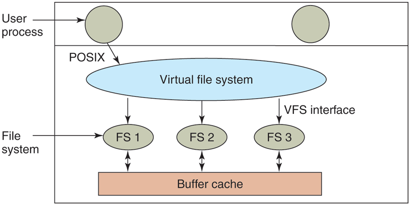
Position of the virtual file system.
All system calls relating to files are directed to the virtual file system for initial processing. These calls, coming from user processes, are the standard POSIX calls, such as open, read, write, lseek, and so on. Thus the VFS has an ‘‘upper’’ interface to user processes and it is the well-known POSIX interface.
The VFS also has a ‘‘lower’’ interface to the concrete file systems, which is labeled VFS interface in Fig. 4-21. This interface consists of several dozen function calls that the VFS can make to each file system to get work done. Thus to create a new file system that works with the VFS, the designers of the new file system must make sure that it supplies the function calls the VFS requires. An obvious example of such a function is one that reads a specific block from disk, puts it in the file system’s buffer cache, and returns a pointer to it. Thus the VFS has two distinct interfaces: the upper one to the user processes and the lower one to the concrete file systems.
While most of the file systems under the VFS represent partitions on a local disk, this is not always the case. In fact, the original motivation for Sun to build the VFS was to support remote file systems using the NFS (Network File System) protocol. The VFS design is such that as long as the concrete file system supplies the functions the VFS requires, the VFS does not know or care where the data are stored or what the underlying file system is like. It requires is the proper interface to the underlying file systems.
Internally, most VFS implementations are essentially object oriented, even if they are written in C rather than C++. There are several key object types that are normally supported. These include the superblock (which describes a file system), the v-node (which describes a file), and the directory (which describes a file system directory). Each of these has associated operations (methods) that the concrete file systems must support. In addition, the VFS has some internal data structures for its own use, including the mount table and an array of file descriptors to keep track of all the open files in the user processes.
To understand how the VFS works, let us run through an example chronologically. When the system is booted, the root file system is registered with the VFS. In addition, when other file systems are mounted, either at boot time or during operation, they too must register with the VFS. When a file system registers, what it basically does is provide a list of the addresses of the functions the VFS requires, either as one long call vector (table) or as several of them, one per VFS object, as the VFS demands. Thus once a file system has registered with the VFS, the VFS knows how to, say, read a block from it—it simply calls the fourth (or whatever) function in the vector supplied by the file system. Similarly, the VFS then also knows how to carry out every other function the concrete file system must supply: it just calls the function whose address was supplied when the file system registered.
After a file system has been mounted, it can be used. For example, if a file system has been mounted on /usr and a process makes the call
open(“/usr/include/unistd.h”, O_RDONLY)while parsing the path, the VFS sees that a new file system has been mounted on /usr and locates its superblock by searching the list of superblocks of mounted file systems. Having done this, it can find the root directory of the mounted file system and look up the path include/unistd.h there. The VFS then creates a v-node and makes a call to the concrete file system to return all the information in the file’s inode. This information is copied into the v-node (in RAM), along with other information, most importantly the pointer to the table of functions to call for operations on v-nodes, such as read, write, close, and so on.
After the v-node has been created, the VFS makes an entry in the file-descriptor table for the calling process and sets it to point to the new v-node. (For the purists, the file descriptor actually points to another data structure that contains the current file position and a pointer to the v-node, but this detail is not important for our purposes here.) Finally, the VFS returns the file descriptor to the caller so it can use it to read, write, and close the file.
Later when the process does a read using the file descriptor, the VFS locates the v-node from the process and file descriptor tables and follows the pointer to the table of functions, all of which are addresses within the concrete file system on which the requested file resides. The function that handles read is now called and code within the concrete file system goes and gets the requested block. The VFS has no idea whether the data are coming from the local disk, a remote file system over the network, a USB stick, or something different. The data structures involved are shown in Fig. 4-22. Starting with the caller’s process number and the file descriptor, successively the v-node, read function pointer, and access function within the concrete file system are located.
Figure 4-22
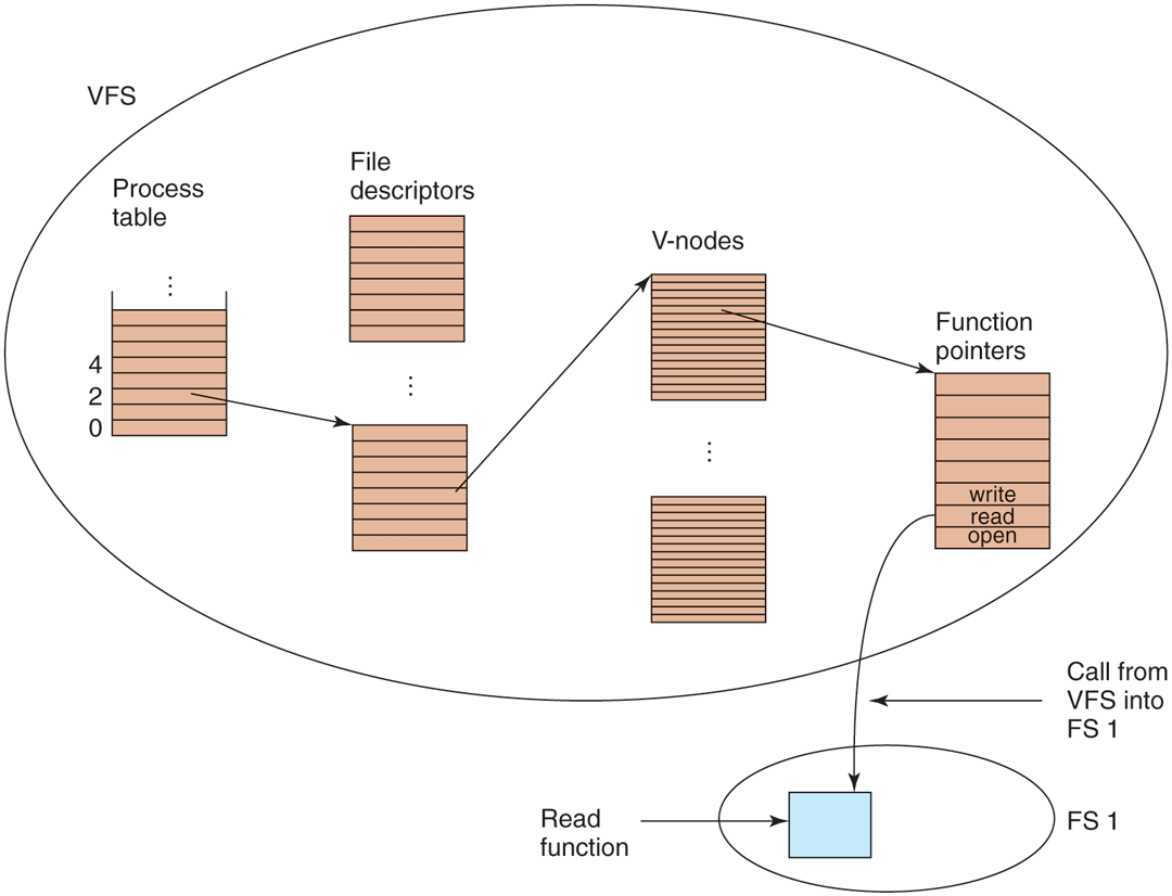
A simplified view of the data structures and code used by the VFS and concrete file system to do a read.
In this manner, it becomes relatively straightforward to add new file systems. To make one, the designers first get a list of function calls the VFS expects and then write their file system to provide all of them. Alternatively, if the file system already exists and needs to be ported to the VFS, then they have to provide wrapper functions that do what the VFS needs, usually by making one or more native calls to the underlying concrete file system.