3.2 A Memory Abstraction: Address Spaces
All in all, exposing physical memory to processes has several major drawbacks. First, if user programs can address every byte of memory, they can easily trash the operating system, intentionally or by accident, bringing the system to a grinding halt (unless there is special hardware like the IBM 360’s lock-and-key scheme). This problem exists even if only one user program (application) is running. Second, with this model, it is difficult to have multiple programs running at once (taking turns, if there is only one CPU). On personal computers, it is common to have several programs open at once (a word processor, an email program, a Web browser), one of them having the current focus, but the others being reactivated at the click of a mouse. Since this situation is difficult to achieve when there is no abstraction from physical memory, something had to be done.
3.2.1 The Notion of an Address Space
Two problems have to be solved to allow multiple applications to be in memory at the same time without interfering with each other: protection and relocation. We looked at a primitive solution to the former used on the IBM 360: label chunks of memory with a protection key and compare the key of the executing process to that of every memory word fetched. However, this approach by itself does not solve the latter problem, although it can be solved by relocating programs as they are loaded, but this is a slow and complicated solution.
A better solution is to invent a new abstraction for memory: the address space. Just as the process concept creates a kind of abstract CPU to run programs, the address space creates a kind of abstract memory for programs to use. An address space is the set of addresses that a process can use to address memory. Each process has its own address space, independent of those of other processes (except in some special circumstances where processes want to share their address spaces).
The concept of an address space is very general and occurs in many contexts. Consider telephone numbers. In the United States and many other countries, a local telephone number is usually a 7-digit number. The address space for telephone numbers thus runs from 0,000,000 to 9,999,999, although some numbers, such as those beginning with 000 are not used. The address space for I/O ports on the x86 runs from 0 to 16383. IPv4 addresses are 32-bit numbers, so their address space runs from 0 to (again, with some reserved numbers).
Address spaces do not have to be numeric. The set of .com Internet domains is also an address space. This address space consists of all the strings of length 2 to 63 characters that can be made using letters, numbers, and hyphens, followed by .com. By now you should get the idea. It is fairly simple.
Somewhat harder is how to give each program its own address space, so address 28 in one program means a different physical location than address 28 in another program. Below we will discuss a simple way that used to be common but has fallen into disuse due to the ability to put much more complicated (and better) schemes on modern CPU chips.
Base and Limit Registers
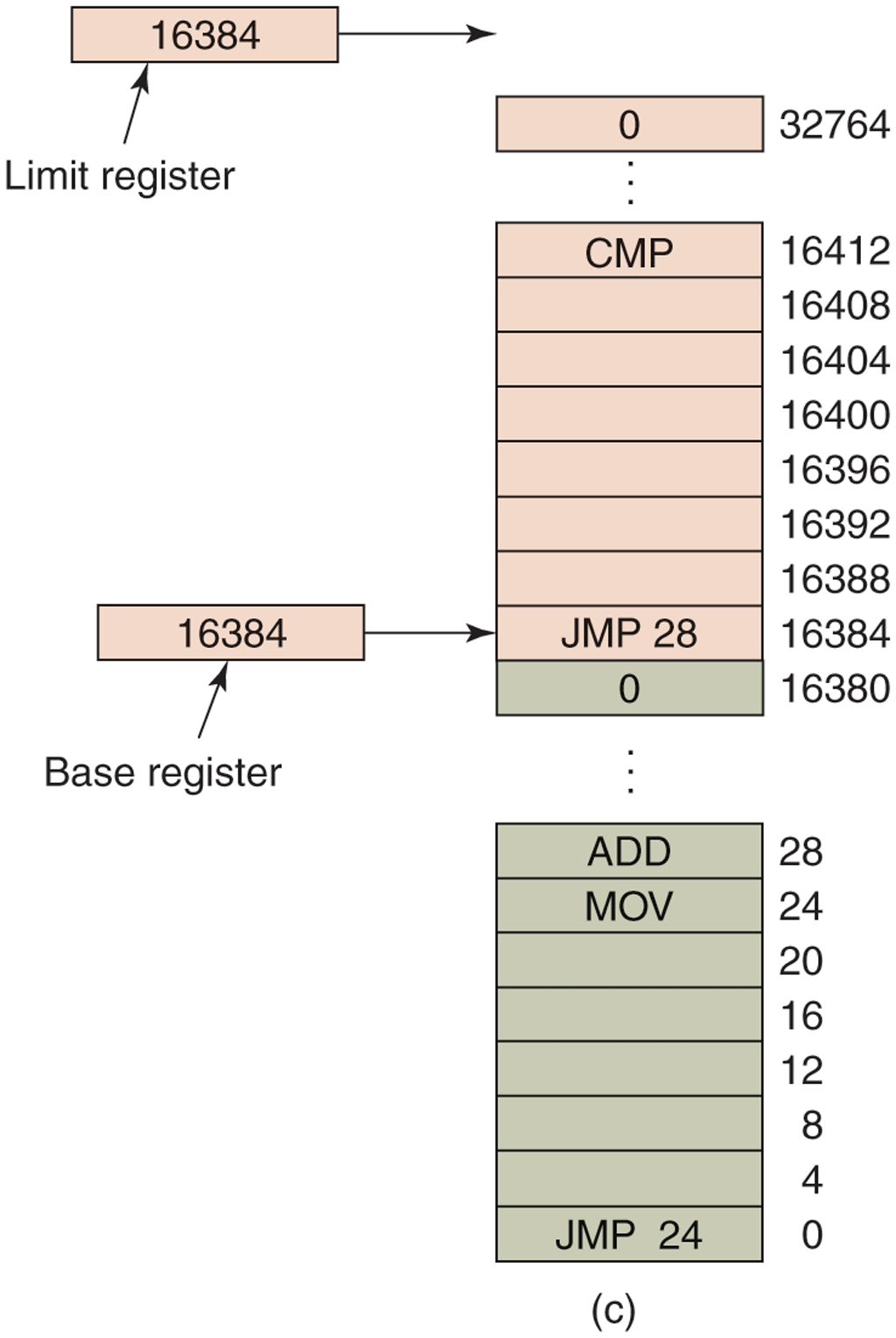
This simple solution uses a particularly simple version of dynamic relocation. What it does is map each process’ address space onto a different part of physical memory in a simple way. The classical solution, which was used on machines ranging from the CDC 6600 (the world’s first supercomputer) to the Intel 8088 (the heart of the original IBM PC), is to equip each CPU with two special hardware registers, usually called the base and limit registers. When these registers are used, programs are loaded into consecutive memory locations wherever there is room and without relocation during loading, as shown in Fig. 3-2(c). When a process is run, the base register is loaded with the physical address where its program begins in memory and the limit register is loaded with the length of the program. In Fig. 3-2(c), the base and limit values that would be loaded into these hardware registers when the first program is run are 0 and 16,384, respectively. The values used when the second program is run are 16,384 and 32,768, respectively. If a third 16-KB program were loaded directly above the second one and run, the base and limit registers would be 32,768 and 16,384.
Every time a process references memory, either to fetch an instruction or read or write a data word, the CPU hardware automatically adds the base value to the address generated by the process before sending the address out on the memory bus. Simultaneously, it checks whether the address offered is equal to or greater than the value in the limit register, in which case a fault is generated and the access is terminated. Thus, in the case of the first instruction of the second program in Fig. 3-2(c), the process executes a
JMP 28instruction, but the hardware treats it as though it were
JMP 16412so it lands on the CMP instruction as expected. The settings of the base and limit registers during the execution of the second program of Fig. 3-2(c) are shown in Fig. 3-3.
Figure 3-3
Base and limit registers can be used to give each process a separate address space.
Using base and limit registers is an easy way to give each process its own private address space because every memory address generated automatically has the base-register contents added to it before being sent to memory. In many implementations, the base and limit registers are protected in such a way that only the operating system can modify them. This was the case on the CDC 6600, but not on the Intel 8088, which did not even have the limit register. It did have multiple base registers, allowing program text and data, for example, to be independently relocated, but offered no protection from out-of-range memory references.
A disadvantage of relocation using base and limit registers is the need to perform an addition and a comparison on every memory reference. Comparisons can be done fast, but additions are slow due to carry-propagation time unless special addition circuits are used.
3.2.2 Swapping
If the physical memory of the computer is large enough to hold all the processes, the schemes described so far will more or less do. But in practice, the total amount of RAM needed by all the processes is often much more than can fit in memory. On a typical Windows, MacOS, or Linux system, something like 50–100 processes or more may be started up as soon as the computer is booted. For example, when a Windows application is installed, it often issues commands so that on subsequent system boots, a process will be started that does nothing except check for updates to the application. Such a process can easily occupy 5–10 MB of memory. Other background processes check for incoming mail, incoming network connections, and many other things. And all this is before the first user program is started. Serious user application programs nowadays, like Photoshop, can require almost a gigabyte just to boot and many gigabytes once they start processing data. Consequently, keeping all processes in memory all the time requires a huge amount of memory and cannot be done if there is insufficient memory.
Two general approaches to dealing with memory overload have been developed over the years. The simplest strategy, called swapping of processes, consists of bringing in each process in its entirety, running it for a while, then putting it back on nonvolatile storage (disk or SSD). Idle processes are mostly stored on nonvolatile storage, so they do not take up any memory when they are not running (although some of them wake up periodically to do their work, then go to sleep again). The other strategy, called virtual memory, allows programs to run even when they are only partially in main memory. Below we will study swapping; in Sec. 3.3 we will examine virtual memory.
The operation of a swapping system is illustrated in Fig. 3-4. Initially, only process A is in memory. Then processes B and C are created or swapped in from nonvolatile storage. In Fig. 3-4(d) A is swapped out to nonvolatile storage. Then D comes in and B goes out. Finally A comes in again. Since A is now at a different location, addresses contained in it must be relocated, either by software when it is swapped in or (more likely) by hardware during program execution. For example, base and limit registers would work fine here.
Figure 3-4
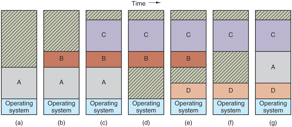
Memory allocation changes as processes come into memory and leave it. The shaded regions are unused memory.
When swapping creates multiple holes in memory, it is possible to combine them all into one big one by moving all the processes downward as far as possible. This technique is known as memory compaction. It is usually not done because it requires a lot of CPU time. For example, on a 16-GB machine that can copy 8 bytes in 8 nsec, it would take about 16 sec to compact all of memory.
A point that is worth making concerns how much memory should be allocated for a process when it is created or swapped in. If processes are created with a fixed size that never changes, then the allocation is simple: the operating system allocates exactly what is needed, no more and no less.
If, however, processes’ data segments can grow, for example, by dynamically allocating memory from a heap, as in many programming languages, a problem occurs whenever a process tries to grow. If a hole is adjacent to the process, it can be allocated and the process allowed to grow into the hole. On the other hand, if the process is adjacent to another process, the growing process will either have to be moved to a hole in memory large enough for it, or one or more processes will have to be swapped out to create a large enough hole. If a process cannot grow in memory and the swap area on the disk or SSD is full, the process will have to suspended until some space is freed up (or it can be killed).
If it is expected that most processes will grow as they run, it is probably a good idea to allocate a little extra memory whenever a process is swapped in or moved, to reduce the overhead associated with moving or swapping processes that no longer fit in their allocated memory. However, when swapping processes to nonvolatile storage, only the memory actually in use should be swapped; it is wasteful to swap the extra memory as well. In Fig. 3-5(a), we see a memory configuration in which space for growth has been allocated to two processes.
Figure 3-5
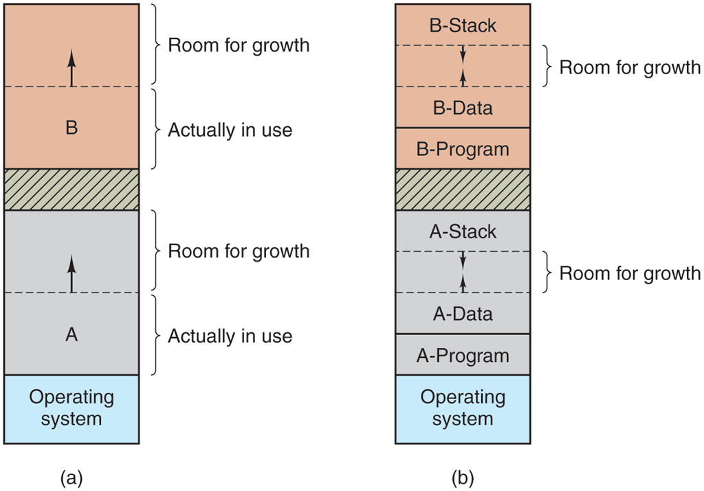
(a) Allocating space for a growing data segment. (b) Allocating space for a growing stack and a growing data segment.
If processes can have two growing segments—for example, the data segment being used as a heap for variables that are dynamically allocated and released and a stack segment for the normal local variables and return addresses—an alternative arrangement suggests itself, namely that of Fig. 3-5(b). In this figure, we see that each process illustrated has a stack at the top of its allocated memory that is growing downward, and a data segment just beyond the program text that is growing upward. The memory between them can be used for either segment. If it runs out, the process will either have to be moved to a hole with sufficient space, swapped out of memory until a large enough hole can be created, or killed.
3.2.3 Managing Free Memory
When memory is assigned dynamically, the operating system must manage it. In general terms, there are two ways to keep track of memory usage: bitmaps and free lists. In this section and the next one, we will look at these two methods. In Chapter 10, we will look at some specific memory allocators used in Linux (like buddy and slab allocators) in more detail. We will also see in later chapters that tracking the usage of resources is not specific to memory management. For instance, file systems also need to keep track of free disk blocks. In fact, keeping track of what slots are free in an set of resources is common in many programs.
Memory Management with Bitmaps
With a bitmap, memory is divided into allocation units as small as a few words and as large as several kilobytes. Corresponding to each allocation unit is a bit in the bitmap, which is 0 if the unit is free and 1 if it is occupied (or vice versa). Figure 3-6(a) shows part of memory and the corresponding bitmap in Fig. 3-6(b).
Figure 3-6
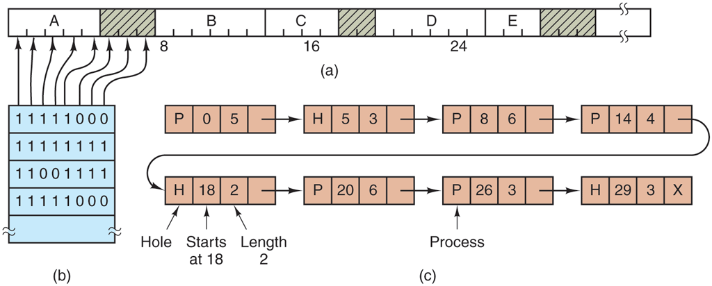
(a) A part of memory with five processes and three holes. The tick marks show the memory allocation units. The shaded regions (0 in the bitmap) are free. (b) The corresponding bitmap. (c) The same information as a list.
The size of the allocation unit is an important design issue. The smaller the allocation unit, the larger the bitmap. However, even with an allocation unit as small as 4 bytes, 32 bits of memory will require only 1 bit of the map. A memory of 32n bits will use n map bits, so the bitmap will take up only 1/32 of memory. If the allocation unit is chosen large, the bitmap will be smaller, but appreciable memory may be wasted in the last unit of the process if the process size is not an exact multiple of the allocation unit.
A bitmap provides a simple way to keep track of memory words in a fixed amount of memory because the size of the bitmap depends only on the size of memory and the size of the allocation unit. The main problem is that when it has been decided to bring a k-unit process into memory, the memory manager must search the bitmap to find a run of k consecutive 0 bits in the map. Searching a bitmap for a run of a given length is a slow operation (because the run may straddle word boundaries in the map); this is an argument against bitmaps.
Memory Management with Linked Lists
Another way of keeping track of memory is to maintain a linked list of allocated and free memory segments, where a segment either contains a process or is an empty hole between two processes. The memory of Fig. 3-6(a) is represented in Fig. 3-6(c) as a linked list of segments. Each entry in the list specifies a hole (H) or process (P), the address at which it starts, the length, and a pointer to the next item.
In this example, the segment list is kept sorted by address. Sorting this way has the advantage that when a process terminates or is swapped out, updating the list is straightforward. A terminating process normally has two neighbors (except when it is at the very top or bottom of memory). These may be either processes or holes, leading to the four combinations shown in Fig. 3-7. In Fig. 3-7(a) updating the list requires replacing a P by an H. In Fig. 3-7(b) and (c), two entries are coalesced into one, and the list becomes one entry shorter. In Fig. 3-7(d), three entries are merged and two items are removed from the list.
Figure 3-7
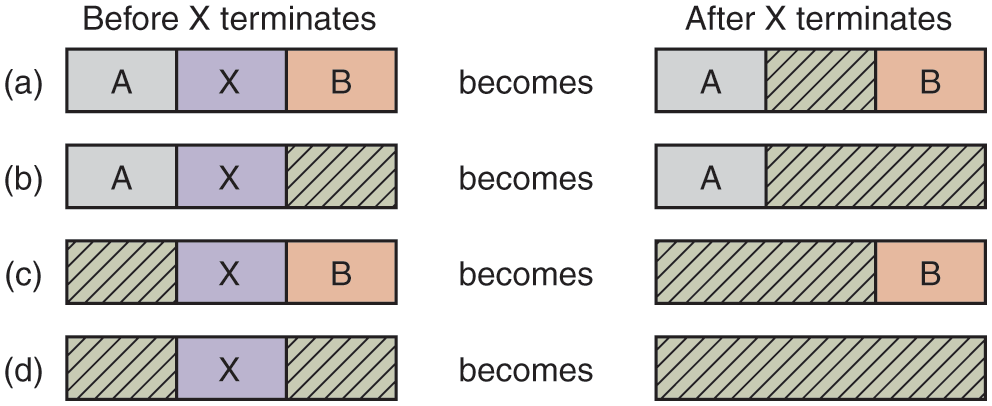
Four neighbor combinations for the terminating process, X.
Since the process table slot for the terminating process will normally point to the list entry for the process itself, it may be more convenient to have the list as a double-linked list, rather than the single-linked list of Fig. 3-6(c). This structure makes it easier to find the previous entry and to see if a merge is possible.
When the processes and holes are kept on a list sorted by address, several algorithms can be used to allocate memory for a created process (or an existing process being swapped in from disk or SSD). We assume that the memory manager knows how much memory to allocate. The simplest algorithm is first fit. The memory manager scans along the list of segments until it finds a hole that is big enough. The hole is then broken up into two pieces, one for the process and one for the unused memory, except in the statistically unlikely case of an exact fit. First fit is a fast algorithm because it searches as little as possible.
A minor variation of first fit is next fit. It works the same way as first fit, except that it keeps track of where it is whenever it finds a suitable hole. The next time it is called to find a hole, it starts searching the list from the place where it left off last time, instead of always at the beginning, as first fit does. Simulations by Bays (1977) show that next fit gives slightly worse performance than first fit.
Another well-known and widely used algorithm is best fit. Best fit searches the entire list, from beginning to end, and takes the smallest hole that is adequate. Rather than breaking up a big hole that might be needed later, best fit tries to find a hole that is close to the actual size needed, to best match the request and the available holes.
As an example of first fit and best fit, consider Fig. 3-6 again. If a block of size 2 is needed, first fit will allocate the hole at 5, but best fit will allocate the hole at 18.
Best fit is slower than first fit because it must search the entire list every time it is called. Somewhat surprisingly, it also results in more wasted memory than first fit or next fit because it tends to fill up memory with tiny, useless holes. First fit generates larger holes on the average.
To get around the problem of breaking up nearly exact matches into a process and a tiny hole, one could think about worst fit, that is, always take the largest available hole, so that the new hole will be big enough to be useful. Simulation has shown that worst fit is not a very good idea either.
All four algorithms can be speeded up by maintaining separate lists for processes and holes. In this way, all of them devote their full energy to inspecting holes, not processes. The inevitable price that is paid for this speedup on allocation is the additional complexity and slowdown when deallocating memory, since a freed segment has to be removed from the process list and inserted into the hole list.
If distinct lists are maintained for processes and holes, the hole list may be kept sorted on size, to make best fit faster. When best fit searches a list of holes from smallest to largest, as soon as it finds a hole that fits, it knows that the hole is the smallest one that will do the job, hence the best fit. No further searching is needed, as it is with the single-list scheme. With a hole list sorted by size, first fit and best fit are equally fast, and next fit is pointless.
When the holes are kept on separate lists from the processes, a small optimization is possible. Instead of having a separate set of data structures for maintaining the hole list, as is done in Fig. 3-6(c), the information can be stored in the holes. The first word of each hole could be the hole size, and the second word a pointer to the following entry. The nodes of the list of Fig. 3-6(c), which require three words and one bit (P/H), are no longer needed.
Yet another allocation algorithm is quick fit, which maintains separate lists for some of the more common sizes requested. For example, it might have a table with n entries, in which the first entry is a pointer to the head of a list of 4-KB holes, the second entry is a pointer to a list of 8-KB holes, the third entry a pointer to 12-KB holes, and so on. Holes of, say, 21 KB, could be put either on the 20-KB list or on a special list of odd-sized holes.
With quick fit, finding a hole of the required size is extremely fast, but it has the same disadvantage as all schemes that sort by hole size, namely, when a process terminates or is swapped out, finding its neighbors to see if a merge with them is possible is quite expensive. If merging is not done, memory will quickly fragment into a large number of small holes into which no processes fit.