Chapter 10

Primes

The following two chapters explain public-key cryptographic systems. This requires some mathematics to get started. It is always tempting to dispense with the understanding and only present the formulas and equations, but we feel very strongly that this is a dangerous thing to do. To use a tool, you should understand the properties of that tool. This is easy with something like a hash function. We have an “ideal” model of a hash function, and we desire the actual hash function to behave like the ideal model. This is not so easy to do with public-key systems because there are no “ideal” models to work with. In practice, you have to deal with the mathematical properties of the public-key systems, and to do that safely you must understand these properties. There is no shortcut here; you must understand the mathematics. Fortunately, the only background knowledge required is high school math.

This chapter is about prime numbers. Prime numbers play an important role in mathematics, but we are interested in them because some of the most important public-key crypto systems are based on prime numbers.

10.1 Divisibility and Primes

A number a is a divisor of b (notation a | b, pronounced “a divides b”) if you can divide b by a without leaving a remainder. For example, 7 is a divisor of 35 so we write 7 | 35. We call a number a prime number if it has exactly two positive divisors, namely 1 and itself. For example, 13 is a prime; the two divisors are 1 and 13. The first few primes are easy to find: 2, 3, 5, 7, 11, 13, …. Any integer greater than 1 that is not prime is called a composite. The number 1 is neither prime nor composite.

We will use the proper mathematical notation and terminology in the chapters ahead. This will make it much easier to read other texts on this subject. The notation might look difficult and complicated at first, but this part of mathematics is really easy.

Here is a simple lemma about divisibility:

Lemma 1 If a | b and b | c then a | c.

Proof

If a | b, then there is an integer s such that as = b. (After all, b is divisible by a so it must be a multiple of a.) And if b | c then there is an integer t such that bt = c. But this implies that c = bt = (as)t = a(st) and therefore a is a divisor of c. (To follow this argument, just verify that each of the equal signs is correct. The conclusion is that the first item c must be equal to the last item a(st).)

The lemma is a statement of fact. The proof argues why the lemma is true. The little square box signals the end of the proof. Mathematicians love to use lots of symbols.1 This is a very simple lemma, and the proof should be easy to follow, as long as you remember what the notation a | b means.

Prime numbers have been studied by mathematicians throughout the ages. Even today, if you want to generate all primes below one million, you should use an algorithm developed just over 2000 years ago by Eratosthenes, a friend of Archimedes. (Eratosthenes was also the first person to accurately measure the diameter of the earth. A mere 1700 years later Columbus allegedly used a much smaller—and wrong—estimate for the size of the earth when he planned to sail to India by going due west.) Euclid, another great Greek mathematician, gave a beautiful proof that showed there are an infinite number of primes. This is such a beautiful proof that we'll include it here. Reading through it will help you reacquaint yourself with the math.

Before we start with the real proof we will give a simple lemma.

Lemma 2 Let n be a positive number greater than 1. Let d be the smallest divisor of n that is greater than 1. Then d is prime.

Proof

First of all, we have to check that d is well defined. (If there is a number n that has no smallest divisor, then d is not properly defined and the lemma is nonsensical.) We know that n is a divisor of n, and n > 1, so there is at least one divisor of n that is greater than 1. Therefore, there must also be a smallest divisor greater than 1.

To prove that d is prime, we use a standard mathematician's trick called reductio ad absurdum or proof by contradiction. To prove a statement X, we first assume that X is not true and show that this assumption leads to a contradiction. If assuming that X is not true leads to a contradiction, then obviously X must be true.

In our case, we will assume that d is not a prime. If d is not a prime, it has a divisor e such that 1 < e < d. But we know from Lemma 1 that if e | d and d | n then e | n, so e is a divisor of n and is smaller than d. But this is a contradiction, because d was defined as the smallest divisor of n. Because a contradiction cannot be true, our assumption must be false, and therefore d must be prime.

Don't worry if you find this type of proof a bit confusing; it takes some getting used to.

We can now prove that there are an infinite number of primes.

Theorem 3 (Euclid) There are an infinite number of primes.

Proof

We again assume the opposite of what we try to prove. Here we assume that the number of primes is finite, and therefore that the list of primes is finite. Let's call them p1, p2, p3, …, pk, where k is the number of primes. We define the number n := p1 p2 p3 pk + 1, which is the product of all our primes plus one.

Consider the smallest divisor greater than 1 of n; we'll call it d again. Now d is prime (by Lemma 2) and d | n. But none of the primes in our finite list of primes is a divisor of n. After all, they are all divisors of n − 1, so if you divide n by one of the pi's in the list, you are always left with a remainder of 1. So d is a prime and it is not in the list. But this is a contradiction, as the list is defined to contain all the primes. Thus, assuming that the number of primes is finite leads to a contradiction. We are left to conclude that the number of primes is infinite.

This is basically the proof that Euclid gave over 2000 years ago.

There are many more results on the distribution of primes, but interestingly enough, there is no easy formula for the exact number of primes in a specific interval. Primes seem to occur fairly randomly. There are even very simple conjectures that have never been proven. For example, the Goldbach conjecture is that every even number greater than 2 is the sum of two primes. This is easy to verify with a computer for relatively small even numbers, but mathematicians still don't know whether it is true for all even numbers.

The fundamental theorem of arithmetic is also useful to know: any integer greater than 1 can be written in exactly one way as the product of primes (if you disregard the order in which you write the primes). For example, 15 = 3 · 5; 255 = 3 · 5 · 17; and 60 = 2 · 2 · 3 · 5. We won't prove this here. Check any textbook on number theory if you want to know the details.

10.2 Generating Small Primes

Sometimes it is useful to have a list of small primes, so here is the Sieve of Eratosthenes, which is still the best algorithm for generating small primes. The 220 in the pseudocode below is a stand-in for any appropriate small constant.

function SMALLPRIMELIST

input:  n      Limit on primes to generate. Must satisfy 2 ≤ n ≤ 220. 

output: P      List of all primes ≤n.

    Limit the size of n. If n is too large we run out of memory. 

    assert 2 ≤ n ≤ 220 

    Initialize a list of flags all set to one.

    (b2,  b3,  …,  bn) ← (1, 1, …, 1)

    i ← 2

    while  i2 ≤ n do

       We have found a prime i. Mark all multiples of i composite.

       for j ∈ 2i,  3i,  4i,  …, n/i i  do

            bj ← 0 

       od

       Look for the next prime in our list. It can be shown that this loop never results 

                 in the condition i > n, which would access a nonexistent bi.

       repeat

           i ← i + 1   bi=1 

    od

    All our primes are now marked with a one. Collect them in a list. 

    P ← []

    for k ∈ 2,  3,  4,  …,  n  do

         if  bk = 1  then

             P ← P || k

         fi

    od

    return P

The algorithm is based on a simple idea. Any composite number c is divisible by a prime that is smaller than c. We keep a list of flags, one for each of the numbers up to n. Each flag indicates whether the corresponding number could be prime. Initially all numbers are marked as potential primes by setting the flag to 1. We start with i being the first prime 2. Of course, none of the multiples of i can be prime so we mark 2i, 3i, 4i, etc. as being composite by setting their flag to 0. We then increment i until we have another candidate prime. Now this candidate is not divisible by any smaller prime, or it would have been marked as a composite already. So the new i must be the next prime. We keep marking the composite numbers and finding the next prime until i2 > n.

It is clear that no prime will ever be marked as a composite, since we only mark a number as a composite when we know a factor of it. (The loop that marks them as composite loops over 2i, 3i, …. Each of these terms has a factor i and therefore cannot be prime.)

Why can we stop when i2 > n? Well, suppose a number k is composite, and let p be its smallest divisor greater than 1. We already know that p is prime (see Lemma 2). Let q := k/p. We now have p ≤ q; otherwise, q would be a divisor of k smaller than p, which contradicts the definition of p. The crucial observation is that , because if p were larger than we would have . This last inequality would show that k > k, which is an obvious fallacy. So .

We have shown that any composite k is divisible by a prime . So any composite ≤n is divisible by a prime . When i2 > n then . But we have already marked the multiples of all the primes less than i as composite in the list, so every composite <n has already been marked as such. The numbers in the list that are still marked as primes are really prime.

The final part of the algorithm simply collects them in a list to be returned.

There are several optimizations you can make to this algorithm, but we have left them out to make things simpler. Properly implemented, this algorithm is very fast.

You might wonder why we need the small primes. It turns out that small primes are useful to generate large primes with, something we will get to soon.

10.3 Computations Modulo a Prime

The main reason why primes are so useful in cryptography is that you can compute modulo a prime.

Let p be a prime. When we compute modulo a prime we only use the numbers 0, 1, …, p − 1. The basic rule for computations modulo a prime is to do the computations using the numbers as integers, just as you normally would, but every time you get a result r you take it modulo p. Taking a modulo is easy: just divide the result r by p, throw away the quotient, and keep the remainder as the answer. For example, if you take 25 modulo 7 you divide 25 by 7, which gives us a quotient of 3 with a remainder of 4. The remainder is the answer, so (25 mod 7) = 4. The notation (a mod b) is used to denote an explicit modulo operation, but modulo computations are used very often, and there are several other notations in general use. Often the entire equation will be written without any modulo operations, and then (mod p) will be added at the end of the equation to remind you that the whole thing is to be taken modulo p. When the situation is clear from the context, even this is left out, and you have to remember the modulo yourself.

You don't need to write parentheses around a modulo computation. We could just as well have written a mod b, but as the modulo operator looks very much like normal text, this can be a bit confusing for people who are not used to it. To avoid confusion we tend to either put (a mod b) in parentheses or write a (mod b), depending on which is clearer in the relevant context.

One word of warning: Any integer taken modulo p is always in the range 0, …, p − 1, even if the original integer is negative. Some programming languages have the (for mathematicians very irritating) property that they allow negative results from a modulo operation. If you want to take −1 modulo p, then the answer is p − 1. More generally: to compute (a mod p), find integers q and r such that a = qp + r and 0 ≤ r < p. The value of (a mod p) is defined to be r. If you fill in a = −1 then you find that q = −1 and r = p − 1.

10.3.1 Addition and Subtraction

Addition modulo p is easy. Just add the two numbers, and subtract p if the result is greater than or equal to p. As both inputs are in the range 0, …, p − 1, the sum cannot exceed 2p − 1, so you have to subtract p at most once to get the result back in the proper range.

Subtraction is similar to addition. Subtract the numbers, and add p if the result is negative.

These rules only work when the two inputs are both modulo p numbers already. If they are outside the range, you have to do a full reduction modulo p.

It takes a while to get used to modulo computations. You get equations like 5 + 3 = 1 (mod 7). This looks odd at first. You know that 5 plus 3 is not 1. But while 5 + 3 = 8 is true in the integer numbers, working modulo 7 we have 8 mod 7 = 1, so 5 + 3 = 1 (mod 7).

We use modulo arithmetic in real life quite often without realizing it. When computing the time of day, we take the hours modulo 12 (or modulo 24). A bus schedule might state that the bus leaves at 55 minutes past the hour and takes 15 minutes. To find out when the bus arrives, we compute 55 + 15 = 10 (mod 60), and determine it arrives at 10 minutes past the hour. For now we will restrict ourselves to computing modulo a prime, but you can do computations modulo any number you like.

One important thing to note is that if you have a long equation like 5 + 2 + 5 + 4 + 6 (mod 7), you can take the modulo at any point in the computation. For example, you could sum up 5 + 2 + 5 + 4 + 6 to get 22, and the compute 22 (mod 7) to get 1. Alternately, you could compute 5 + 2(mod 7) to get 0, then compute 0 + 5(mod 7) to get 5, and then 5 + 4(mod 7) to get 2, and then 2 + 6 (mod 7) to get 1.

10.3.2 Multiplication

Multiplication is, as always, more work than addition. To compute (ab mod p) you first compute ab as an integer, and then take the result modulo p. Now ab can be as large as (p − 1)2 = p2 − 2p + 1. Here you have to perform a long division to find (q, r) such that ab = qp + r and 0 ≤ r < p. Throw away the q; the r is the answer.

Let's give you an example: Let p = 5. When we compute 3 · 4 (mod p) the result is 2. After all, 3 · 4 = 12, and (12 mod 5) = 2. So we get 3 · 4 = 2 (mod p).

As with addition, you can compute the modulus all at once or iteratively. For example, given a long equation 3 · 4 · 2 · 3 (mod p), you can compute 3 · 4 · 2 · 3 = 72 and then compute (72 mod 5) = 2. Or you could compute (3 · 4 mod 5) = 2, then (2 · 2 mod 5) = 4, and then (4 · 3 mod 5) = 2.

10.3.3 Groups and Finite Fields

Mathematicians call the set of numbers modulo a prime p a finite field and often refer to it as the “mod p” field, or simply “mod p.” Here are some useful reminders about computations in a mod p field:

• You can always add or subtract any multiple of p from your numbers without changing the result.
• All results are always in the range 0, 1, …, p − 1.
• You can think of it as doing your entire computation in the integers and only taking the modulo at the very last moment. So all the algebraic rules you learned about the integers (such as a(b + c) = ab + ac) still apply.

The finite field of the integers modulo p is referred to using different notations in different books. We will use the notation p to refer to the finite field modulo p. In other texts you might see GF(p) or even /p.

We also have to introduce the concept of a group—another mathematical term, but a simple one. A group is simply a set of numbers together with an operation, such as addition or multiplication.2 The numbers in p form a group together with addition. You can add any two numbers and get a third number in the group. If you want to use multiplication in a group you cannot use the 0. (This has to do with the fact that multiplying by 0 is not very interesting, and that you cannot divide by 0.) However, the numbers 1, …, p − 1 together with multiplication modulo p form a group. This group is called the multiplicative group modulo p and is written in various ways; we will use the notation . A finite field consists of two groups: the addition group and the multiplication group. In the case of p the finite field consists of the addition group, defined by addition modulo p, and the multiplication group .

A group can contain a subgroup. A subgroup consists of some of the elements of the full group. If you apply the group operation to two elements of the subgroup, you again get an element of the subgroup. That sounds complicated, so here is an example. The numbers modulo 8 together with addition (modulo 8) form a group. The numbers {0, 2, 4, 6} form a subgroup. You can add any two of these numbers modulo 8 and get another element of the subgroup. The same goes for multiplicative groups. The multiplicative subgroup modulo 7 consists of the numbers 1, …, 6, and the operation is multiplication modulo 7. The set {1, 6} forms a subgroup, as does the set {1, 2, 4}. You can check that if you multiply any two elements from the same subgroup modulo 7, you get another element from that subgroup.

We use subgroups to speed up certain cryptographic operations. They can also be used to attack systems, which is why you need to know about them.

So far we've only talked about addition, subtraction, and multiplication modulo a prime. To fully define a multiplicative group you also need the inverse operation of multiplication: division. It turns out that you can define division on the numbers modulo p. The simple definition is that a/b (mod p) is a number c such that c · b = a (mod p). You cannot divide by zero, but it turns out that the division a/b (mod p) is always well defined as long as b ≠ 0.

So how do you compute the quotient of two numbers modulo p? This is more complicated, and it will take a few pages to explain. We first have to go back more than 2000 years to Euclid again, and to his algorithm for the GCD.

10.3.4 The GCD Algorithm

Another high-school math refresher course: The greatest common divisor (or GCD) of two numbers a and b is the largest k such that k | a and k | b. In other words, gcd(a, b) is the largest number that divides both a and b.

Euclid gave an algorithm for computing the GCD of two numbers that is still in use today, thousands of years later. For a detailed discussion of this algorithm, see Knuth [75].

Why would this work? The first observation is that the assignment does not change the set of common divisors of a and b. After all, (b mod a) is just b − sa for some integer s. Any number k that divides both a and b will also divide both a and (b mod a). (The converse is also true.) And when a = 0, then b is a common divisor of a and b, and b is obviously the largest such common divisor. You can check for yourself that the loop must terminate because a and b keep getting smaller and smaller until they reach zero.

Let's compute the GCD of 21 and 30 as an example. We start with (a, b) = (21, 30). In the first iteration we compute (30 mod 21) = 9, so we get (a, b) = (9, 21). In the next iteration we compute (21 mod 9) = 3, so we get (a, b) = (3, 9). In the final iteration we compute (9 mod 3) = 0 and get (a, b) = (0, 3). The algorithm will return 3, which is indeed the greatest common divisor of 21 and 30.

The GCD has a cousin: the LCM or least common multiple. The LCM of a and b is the smallest number that is both a multiple of a and a multiple of b. For example, lcm(6, 8) = 24. The GCD and LCM are tightly related by the equation

which we won't prove here but just state as a fact.

10.3.5 The Extended Euclidean Algorithm

This still does not help us to compute division modulo p. For that, we need what is called the extended Euclidean algorithm. The idea is that while computing gcd(a, b) we can also find two integers u and v such that gcd(a, b) = ua + vb. This will allow us to compute a/b (mod p).

This algorithm is very much like the GCD algorithm. We introduce new variables c and d instead of using a and b because we need to refer to the original a and b in our invariant. If you only look at c and d, this is exactly the GCD algorithm. (We've rewritten the d mod c formula slightly, but this gives the same result.) We have added four variables that maintain the given invariant; for each value of c or d that we generate, we keep track of how to express that value as a linear combination of a and b. For the initialization this is easy, as c is initialized to a and d to b. When we modify c and d in the loop it is not terribly difficult to update the u and v variables.

Why bother with the extended Euclidean algorithm? Well, suppose we want to compute 1/b mod p where 1 ≤ b < p. We use the extended Euclidean algorithm to compute EXTENDEDGCD(b, p). Now, we know that the GCD of b and p is 1, because p is prime and it therefore has no other suitable divisors. But the EXTENDEDGCD function also provides two numbers u and v such that ub + vp = gcd(b, p) = 1. In other words, ub = 1 − vp or ub = 1 (mod p). This is the same as saying that u = 1/b (mod p), the inverse of b modulo p. The division a/b can now be computed by multiplying a by u, so we get a/b = au (mod p), and this last formula is something that we know how to compute.

The extended Euclidean algorithm allows us to compute an inverse modulo a prime, which in turn allows us to compute a division modulo p. Together with the addition, subtraction, and multiplication modulo p, this allows us to compute all four elementary operations in the finite field modulo p.

Note that u could be negative, so it is probably a good idea to reduce u modulo p before using it as the inverse of b.

If you look carefully at the EXTENDEDGCD algorithm, you'll see that if you only want u as output, you can leave out the vc and vd variables, as they do not affect the computation of u. This slightly reduces the amount of work needed to compute a division modulo p.

10.3.6 Working Modulo 2

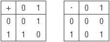
An interesting special case is computation modulo 2. After all, 2 is a prime, so we should be able to compute modulo it. If you've done any programming this might look familiar to you. The addition and multiplication tables modulo 2 are shown in Figure 10.1. Addition modulo 2 is exactly the exclusive-or (XOR) function you find in programming languages. Multiplication is just a simple AND operation. In the field modulo 2 there is only one inversion possible (1/1 = 1) so division is the same operation as multiplication. It shouldn't surprise you that the field 2 is an important tool to analyze certain algorithms used by computers.

10.4 Large Primes

Several cryptographic primitives use very large primes, and we're talking about many hundreds of digits here. Don't worry, you won't have to compute with these primes by hand. That's what the computer is for.

To do any computations at all with numbers this large, you need a multiprecision library. You cannot use floating-point numbers, because they do not have several hundred digits of precision. You cannot use normal integers, because in most programming languages they are limited to a dozen digits or so. Few programming languages provide native support for arbitrary precision integers. Writing routines to perform computations with large integers is fascinating. For a good overview, see Knuth [75, Section 4.3]. However, implementing a multiprecision library is far more work than you might expect. Not only do you have to get the right answer, but you always strive to compute it as quickly as possible. There are quite a number of special situations you have to deal with carefully. Save your time for more important things, and download one of the many free libraries from the Internet, or use a language like Python that has built-in large integer support.

For public-key cryptography, the primes we want to generate are 2000–4000 bits long. The basic method of generating a prime that large is surprisingly simple: take a random number and check whether it is prime. There are very good algorithms to determine whether a large number is prime or not. There are also very many primes. In the neighborhood of a number n, approximately one in every lnn numbers is prime. (The natural logarithm of n, or lnn for short, is one of the standard functions on any scientific calculator. To give you an idea of how slowly the logarithm grows when applied to large inputs: the natural logarithm of 2k is slightly less than 0.7 · k.) A number that is 2000 bits long falls between 21999 and 22000. In that range, about one in every 1386 of the numbers is prime. And this includes a lot of numbers that are trivially composite, such as the even numbers.

Generating a large prime looks something like this:

function GENERATELARGEPRIME

input:  l     Lower bound of range in which prime should lie. 

        u     Upper bound of range in which prime should lie. 

output: p     A random prime in the interval l, …,  u

    Check for a sensible range. 

    assert 2 < l ≤ u

    Compute maximum number of attempts

    r ← 100 (log2 u + 1) 

    repeat

        r ← r − 1

        assert r > 0  

        Choose n randomly in the right interval

        n ∈  l, …,  u

        Continue trying until we find a prime.

    until ISPRIME(n)  

    return n

We use the operator ∈ to indicate a random selection from a set. Of course, this requires some output from the PRNG.

The algorithm is relatively straightforward. We first check that we get a sensible interval. The cases l ≤ 2 and l ≥ u are not useful and lead to problems. Note the boundary condition: the case l = 2 is not allowed.3 Next we compute how many attempts we are going to make to find a prime. There are intervals that do not contain a prime. For example, the interval 90, …, 96 is prime-free. A proper program should never hang, independent of its inputs, so we limit the number of tries and generate a failure if we exceed this number. How many times should we try? As stated before, in the neighborhood of u about one in every 0.7 log2 u numbers is prime. (The function log2 is the logarithm to the base 2. The simplest definition is that log2(x) := lnx/ln2). The number log2 u is difficult to compute but log2 u + 1 is much easier; it is the number of bits necessary to represent u as a binary number. So if u is an integer that is 2017 bits long, then log2 u + 1 = 2017. The factor 100 ensures that it is extremely unlikely that we will not find a prime. For large enough intervals, the probability of a failure due to bad luck is less than 2−128, so we can ignore this risk. At the same time, this limit does ensure that the GENERATELARGEPRIME function will terminate. We've been a bit sloppy in our use of an assertion to generate the failure; a proper implementation would generate an error with explanations of what went wrong.

The main loop is simple. After the check that limits the number of tries, we choose a random number and check whether it is prime using the ISPRIME function. We will define this function shortly.

Make sure that the number n you choose is uniformly random in the range l, …, u. Also make sure that the range is not too small if you want your prime to be a secret. If the attacker knows the interval you use, and there are fewer than 2128 primes in that interval, the attacker could potentially try them all.

If you wish, you can make sure the random number you generate is odd by setting the least significant bit just after you generate a candidate n. As 2 is not in your interval, this will not affect the probability distribution of primes you are choosing, and it will halve the number of attempts you have to make. But this is only safe if u is odd; otherwise, setting the least significant bit might bump n just outside the allowed range. Also, this will generate some small bias away from l if l is odd.

The ISPRIME function is a two-step filter. The first phase is a simple test where we try to divide n by all the small primes. This will quickly weed out the great majority of numbers that are composite and divisible by a small prime. If we find no divisors, we employ a heavyweight test called the Rabin-Miller test.

If you are lazy and don't want to generate the small primes, you can cheat a bit. Instead of trying all the primes, you can try 2 and all odd numbers 3, 5, 7, …, 999, in that order. This sequence contains all the primes below 1000, but it also contains a lot of useless composite numbers. The order is important to ensure that a small composite number like 9 is properly detected as being composite. The bound of 1000 is arbitrary and can be chosen for optimal performance.

All that remains to explain is the mysterious Rabin-Miller test that does the hard work.

10.4.1 Primality Testing

It turns out to be remarkably easy to test whether a number is prime. At least, it is remarkably easy compared to factoring a number and finding its prime divisors. These easy tests are not perfect. They are all probabilistic. There is a certain chance they give the wrong answer. By repeatedly running the same test we can reduce the probability of error to an acceptable level.

The primality test of choice is the Rabin-Miller test. The mathematical basis for this test is well beyond the scope of this book, although the outline is fairly simple. The purpose of this test is to determine whether an odd integer n is prime. We choose a random value a less than n, called the basis, and check a certain property of a modulo n that always holds when n is prime. However, you can prove that when n is not a prime, this property holds for at most 25% of all possible basis values. By repeating this test for different random values of a, you build your confidence in the final result. If n is a prime, it will always test as a prime. If n is not a prime, then at least 75% of the possible values for a will show so, and the chance that n will pass multiple tests can be made as small as you want. We limit the probability of a false result to 2−128 to achieve our required security level.

Here is how it goes:

This algorithm only works for an odd n greater or equal to 3, so we test that first. The ISPRIME function should only call this function with a suitable argument, but each function is responsible for checking its own inputs and outputs. You never know how the software will be changed in future.

The basic idea behind the test is known as Fermat's little theorem.4 For any prime n and for all 1 ≤ a < n, the relation an−1 mod n = 1 holds. To fully understand the reasons for this requires more math than we will explain here. A simple test (also called the Fermat primality test) verifies this relation for a number of randomly chosen a values. Unfortunately, there are some obnoxious numbers called the Carmichael numbers. These are composite but they pass the Fermat test for (almost) all basis a.

The Rabin-Miller test is a variation of the Fermat test. First we write n − 1 as 2ts, where s is an odd number. If you want to compute an−1 you can first compute as and then square the result t times to get . Now if as = 1 (mod n) then repeated squaring will not change the result so we have an−1 = 1 (mod n). If as ≠ 1 (mod n), then we look at the numbers (all modulo n, of course). If n is a prime, then we know that the last number must be 1. If n is a prime, then the only numbers that satisfy x2 = 1 (mod n) are 1 and n − 1.5 So if n is prime, then one of the numbers in the sequence must be n − 1, or we could never have the last number be equal to 1. This is really all the Rabin-Miller test checks. If any choice of a demonstrates that n is composite, we return immediately. If n continues to test as a prime, we repeat the test for different a values until the probability that we have generated a wrong answer and claimed that a composite number is actually prime is less than 2−128.

If you apply this test to a random number, the probability of failure of this test is much, much smaller than the bound we use. For almost all composite numbers n, almost all basis values will show that n is composite. You will find a lot of libraries that depend on this and perform the test for only 5 or 10 bases or so. This idea is fine, though we would have to investigate how many attempts are needed to reach an error level of 2−128 or less. But it only holds as long as you apply the ISPRIME test to randomly chosen numbers. Later on we will encounter situations where we apply the primality test to numbers that we received from someone else. These might be maliciously chosen, so the ISPRIME function must achieve a 2−128 error bound all by itself.

Doing the full 64 Rabin-Miller tests is necessary when we receive the number to be tested from someone else. It is overkill when we try to generate a prime randomly. But when generating a prime, you spend most of your time rejecting composite numbers. (Almost all composite numbers are rejected by the very first Rabin-Miller test that you do.) As you might have to try hundreds of numbers before you find a prime, doing 64 tests on the final prime is only marginally slower than doing 10 of them.

In an earlier version of this chapter, the Rabin-Miller routine had a second argument that could be used to select the maximum error probability. But it was a perfect example of a needless option, so we removed it. Always doing a good test to a 2−128 bound is simpler, and much less likely to be improperly used.

There is still a chance of 2−128 that our ISPRIME function will give you the wrong answer. To give you an idea of how small this chance actually is, the chance that you will be killed by a meteorite while you read this sentence is far larger. Still alive? Okay, so don't worry about it.

10.4.2 Evaluating Powers

The Rabin-Miller test spends most of its time computing as mod n. You cannot compute as first and then take it modulo n. No computer in the world has enough memory to even store as, much less the computing power to compute it; both a and s can be thousands of bits long. But we only need as mod n; we can apply the mod n to all the intermediate results, which stops the numbers from growing too large.

There are several ways of computing as mod n, but here is a simple description. To compute as mod n, use the following rules:

• If s = 0 the answer is 1.
• If s > 0 and s is even, then first compute y := as/2 mod n using these very same rules. The answer is given by as mod n = y2 mod n.
• If s > 0 and s is odd, then first compute y := a(s−1)/2 mod n using these very same rules. The answer is given by as mod n = a · y2 mod n.

This is a recursive formulation of the so-called binary algorithm. If you look at the operations performed, it builds up the desired exponent bit by bit from the most significant part of the exponent down to the least significant part. It is also possible to convert this from a recursive algorithm to a loop.

How many multiplications are required to compute as mod n? Let k be the number of bits of s; i.e., 2k−1 ≤ s < 2k. Then this algorithm requires at most 2k multiplications modulo n. This is not too bad. If we are testing a 2000-bit number for primality, then s will also be about 2000 bits long, and we only need 4000 multiplications. That is still a lot of work, but certainly within the capabilities of most desktop computers.

Many public-key cryptographic systems make use of modular exponentiations like this. Any good multiprecision library will have an optimized routine for evaluating modular exponentiations. A special type of multiplication called Montgomery multiplication is well suited for this task. There are also ways of computing as using fewer multiplications [18]. Each of these tricks can save 10%–30% of the time it takes to compute a modular exponentiation, so used in combination they can be important.

Straightforward implementations of modular exponentiation are often vulnerable to timing attacks. See Section 15.3 for details and possible remedies.

10.5 Exercises

Exercise 10.1 Implement SMALLPRIMELIST. What is the worst-case performance of SMALLPRIMELIST? Generate a graph of the timings for your implementation and n = 2, 4, 8, 16, …, 220.

Exercise 10.2 Compute 13635 + 16060 + 8190 + 21363 (mod 29101) in two ways and verify the equivalence: by reducing modulo 29101 after each addition and by computing the entire sum first and then reducing modulo 29101.

Exercise 10.3 Compute the result of 12358 · 1854 · 14303 (mod 29101) in two ways and verify the equivalence: by reducing modulo 29101 after each multiplication and by computing the entire product first and then reducing modulo 29101.

Exercise 10.4 Is {1, 3, 4} a subgroup of the multiplicative group of integers modulo 7?

Exercise 10.5 Use the GCD algorithm to compute the GCD of 91261 and 117035.

Exercise 10.6 Use the EXTENDEDGCD algorithm to compute the inverse of 74 modulo the prime 167.

Exercise 10.7 Implement GENERATELARGEPRIME using a language or library that supports big integers. Generate a prime within the range l = 2255 and u = 2256 − 1.

Exercise 10.8 Give pseudocode for the exponentiation routine described in Section 10.4.2. Your pseudocode should not be recursive but should instead use a loop.

Exercise 10.9 Compute 2735 (mod 569) using the exponentiation routine described in Section 10.4.2. How many multiplications did you have to perform?

1 Using symbols has advantages and disadvantages. We'll use whatever we think is most appropriate for this book.

2 There are a couple of further requirements, but they are all met by the groups we will be talking about.

3 The Rabin-Miller algorithm we use below does not work well when it gets 2 as an argument. That's okay, we already know that 2 is prime so we don't have to generate it here.

4 There are several theorems named after Fermat. Fermat's last Theorem is the most famous one, involving the equation an + bn = cn and a proof too large to fit in the margin of the page.

5 It is easy to check that (n − 1)2 = 1 (mod n).