9

REAPING REWARD BY INCREASING RISK

Theories that are right only 50 percent of the time are less economical than coin-flipping.

— George J. Stigler, The Theory of Price

AS EVERY READER should know by now, risk has its rewards. Thus, both within academia and on the Street, there has long been a scramble to exploit risk to earn greater returns. That’s what this chapter covers: the creation of analytical tools to measure risk and, with such knowledge, reap greater rewards.

We begin with a refinement to modern portfolio theory. As I mentioned in the last chapter, diversification cannot eliminate all risk—as it did in my mythical island economy—because all stocks tend to move up and down together. Thus, diversification in practice reduces some but not all risk. Three academics—the former Stanford professor William Sharpe and the late finance specialists John Lintner and Fischer Black—focused their intellectual energies on determining what part of a security’s risk can be eliminated by diversification and what part cannot. The result is known as the capital-asset pricing model. Sharpe received a Nobel Prize for his contribution to this work at the same time Markowitz was honored in 1990.

The basic logic behind the capital-asset pricing model is that there is no premium for bearing risks that can be diversified away. Thus, to get a higher average long-run rate of return, you need to increase the risk level of the portfolio that cannot be diversified away. According to this theory, savvy investors can outperform the overall market by adjusting their portfolios with a risk measure known as beta.

BETA AND SYSTEMATIC RISK

Beta? How did a Greek letter enter this discussion? Surely it didn’t originate with a stockbroker. Can you imagine any stockbroker saying, “We can reasonably describe the total risk of any security (or portfolio) as the total variability (variance or standard deviation) of the returns from the security”? But we who teach say such things often. We go on to say that part of total risk or variability may be called the security’s systematic risk and that this arises from the basic variability of stock prices in general and the tendency for all stocks to go along with the general market, at least to some extent. The remaining variability in a stock’s returns is called unsystematic risk and results from factors peculiar to that particular company—for example, a strike, the discovery of a new product, and so on.

Systematic risk, also called market risk, captures the reaction of individual stocks (or portfolios) to general market swings. Some stocks and portfolios tend to be very sensitive to market movements. Others are more stable. This relative volatility or sensitivity to market moves can be estimated on the basis of the past record, and is popularly known by—you guessed it—the Greek letter beta.

You are now about to learn all you ever wanted to know about beta but were afraid to ask. Basically, beta is the numerical description of systematic risk. Despite the mathematical manipulations involved, the basic idea behind the beta measurement is one of putting some precise numbers on the subjective feelings money managers have had for years. The beta calculation is essentially a comparison between the movements of an individual stock (or portfolio) and the movements of the market as a whole.

The calculation begins by assigning a beta of 1 to a broad market index. If a stock has a beta of 2, then on average it swings twice as far as the market. If the market goes up 10 percent, the stock tends to rise 20 percent. If a stock has a beta of 0.5, it tends to go up or down 5 percent when the market rises or declines 10 percent. Professionals call high-beta stocks aggressive investments and label low-beta stocks as defensive.

Now, the important thing to realize is that systematic risk cannot be eliminated by diversification. It is precisely because all stocks move more or less in tandem (a large share of their variability is systematic) that even diversified stock portfolios are risky. Indeed, if you diversified perfectly by buying a share in a total stock market index (which by definition has a beta of 1), you would still have quite variable (risky) returns because the market as a whole fluctuates widely.

Unsystematic risk (also called specific or idiosyncratic risk) is the variability in stock prices (and, therefore, in returns from stocks) that results from factors peculiar to an individual company. Receipt of a large new contract, the finding of mineral resources, labor difficulties, accounting fraud, the discovery that the corporation’s treasurer has had his hand in the company till—all can make a stock’s price move independently of the market. The risk associated with such variability is precisely the kind that diversification can reduce. The whole point of portfolio theory is that, to the extent that stocks don’t always move in tandem, variations in the returns from any one security tend to be washed away by complementary variation in the returns from others.

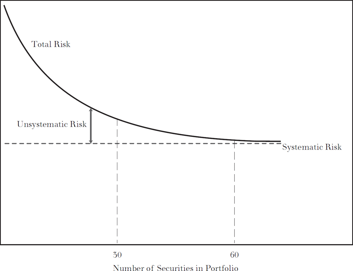
The chart on page 209, similar to the one on page 199, illustrates the important relationship between diversification and total risk. Suppose we randomly select securities for our portfolio that on average are just as volatile as the market (the average betas for the securities in our portfolio will be equal to 1). The chart shows that as we add more securities, the total risk of our portfolio declines, especially at the start.

When thirty securities are selected for our portfolio, a good deal of the unsystematic risk is eliminated, and additional diversification yields little further risk reduction. By the time sixty well-diversified securities are in the portfolio, the unsystematic risk is substantially eliminated and our portfolio (with a beta of 1) will tend to move up and down essentially in tandem with the market. Of course, we could perform the same experiment with stocks whose average beta is 1½. Again, we would find that diversification quickly reduced unsystematic risk, but the remaining systematic risk would be larger. A portfolio of sixty or more stocks with an average beta of 1½ would tend to be 50 percent more volatile than the market.

HOW DIVERSIFICATION REDUCES RISK:RISK OF PORTFOLIO (STANDARD DEVIATION OF RETURN)

Now comes the key step in the argument. Financial theorists and practitioners agree that investors should be compensated for taking on more risk with a higher expected return. Stock prices must, therefore, adjust to offer higher returns where more risk is perceived, to ensure that all securities are held by someone. Obviously, risk-averse investors wouldn’t buy securities with extra risk without the expectation of extra reward. But not all of the risk of individual securities is relevant in determining the premium for bearing risk. The unsystematic part of the total risk is easily eliminated by adequate diversification. So there is no reason to think that investors will receive extra compensation for bearing unsystematic risk. The only part of total risk that investors will get paid for bearing is systematic risk, the risk that diversification cannot help. Thus, the capital-asset pricing model says that returns (and, therefore, risk premiums) for any stock (or portfolio) will be related to beta, the systematic risk that cannot be diversified away.

THE CAPITAL-ASSET PRICING MODEL (CAPM)

The proposition that risk and reward are related is not new. Finance specialists have agreed for years that investors do need to be compensated for taking on more risk. What is different about the new investment technology is the definition and measurement of risk. Before the advent of the capital-asset pricing model, it was believed that the return on each security was related to the total risk inherent in that security. It was believed that the return from a security varied with the variability or standard deviation of the returns it produced. The new theory says that the total risk of each individual security is irrelevant. It is only the systematic component that counts as far as extra rewards go.

Although the mathematical proof of this proposition is forbidding, the logic behind it is fairly simple. Consider two groups of securities—Group I and Group II—with sixty securities in each. Suppose that the systematic risk (beta) for each security is 1; that is, each of the securities in the two groups tends to move up and down in tandem with the general market. Now suppose that, because of factors peculiar to the individual securities in Group I, the total risk for each of them is substantially higher than the total risk for each security in Group II. Imagine, for example, that in addition to general market factors the securities in Group I are also particularly susceptible to climatic variations, to changes in exchange rates, and to natural disasters. The specific risk for each of the securities in Group I will, therefore, be very high. The specific risk for each of the securities in Group II, however, is assumed to be very low, and, hence, the total risk for each of them will be very low. Schematically, this situation appears as follows:

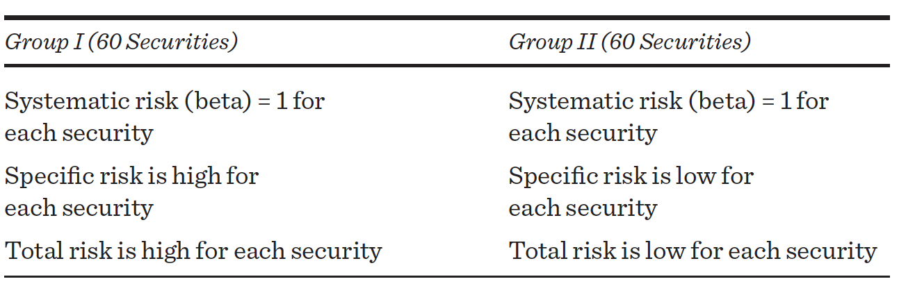
Now, according to the old theory, commonly accepted before the advent of the capital-asset pricing model, returns should be higher for a portfolio made up of Group I securities, because each security in Group I has a higher total risk than each security in Group II, and risk, as we know, has its reward. With a wave of their intellectual wands, the academics changed that sort of thinking. Under the capital-asset pricing model, returns from the two portfolios should be equal. Why?

First, remember the preceding chart on page 209. (The forgetful can take another look.) There we saw that as the number of securities in the portfolio approached sixty, the total risk of the portfolio was reduced to its systematic level. The conscientious reader will now note that in the schematic illustration, the number of securities in each portfolio is sixty. All unsystematic risk has essentially been washed away: An unexpected weather calamity is balanced by a favorable exchange rate, and so forth. What remains is only the systematic risk of each stock in the portfolio, which is given by its beta. But in these two groups, each of the stocks has a beta of 1. Hence, a portfolio of Group I securities and a portfolio of Group II securities will perform exactly the same with respect to risk (standard deviation), even though the stocks in Group I display higher total risk than the stocks in Group II.

The old and the new views now meet head on. Under the old system of valuation, Group I securities were regarded as offering a higher return because of their greater risk. The capital-asset pricing model says there is no greater risk in holding Group I securities if they are in a diversified portfolio. Indeed, if the securities of Group I did offer higher returns, then all rational investors would prefer them over Group II securities and would attempt to rearrange their holdings to capture the higher returns from Group I. But by this very process, they would bid up the prices of Group I securities and push down the prices of Group II securities until, with the attainment of equilibrium (when investors no longer want to switch from security to security), the portfolios for each group had identical returns, related to the systematic component of their risk (beta) rather than to their total risk (including the unsystematic or specific portions). Because stocks can be combined in portfolios to eliminate specific risk, only the undiversifiable or systematic risk will command a risk premium. Investors will not get paid for bearing risks that can be diversified away. This is the basic logic behind the capital-asset pricing model.

In a big fat nutshell, the proof of the capital-asset pricing model (henceforth to be known as CAPM because we economists love to use letter abbreviations) can be stated as follows: If investors did get an extra return (a risk premium) for bearing unsystematic risk, it would turn out that diversified portfolios made up of stocks with large amounts of unsystematic risk would give larger returns than equally risky portfolios of stocks with less unsystematic risk. Investors would snap at the chance to have these higher returns, bidding up the prices of stocks with large unsystematic risk and selling stocks with equivalent betas but lower unsystematic risk. This process would continue until the prospective returns of stocks with the same betas were equalized and no risk premium could be obtained for bearing unsystematic risk. Any other result would be inconsistent with the existence of an efficient market.

The key relationship of the theory is shown in the following diagram. As the systematic risk (beta) of an individual stock (or portfolio) increases, so does the return an investor can expect. If an investor’s portfolio has a beta of zero, as might be the case if all her funds were invested in a government-guaranteed bank savings certificate (beta would be zero because the returns from the certificate would not vary at all with swings in the stock market), the investor would receive some modest rate of return, which is generally called the risk-free rate of interest. As the individual takes on more risk, however, the return should increase. If the investor holds a portfolio with a beta of 1 (as, for example, holding a share in a broad stock-market index fund), her return will equal the general return from common stocks. This return has over long periods of time exceeded the risk-free rate of interest, but the investment is a risky one. In certain periods, the return is much less than the risk-free rate and involves taking substantial losses. This is precisely what is meant by risk.

The diagram shows that a number of different expected returns are possible simply by adjusting the beta of the portfolio. For example, suppose the investor put half of her money in a savings certificate and half in a share of an index fund representing the broad stock market. In this case, she would receive a return midway between the risk-free return and the return from the market, and her portfolio would have an average beta of 0.5.^* The CAPM then asserts that to get a higher average long-run rate of return, you should just increase the beta of your portfolio. An investor can get a portfolio with a beta larger than 1 either by buying high-beta stocks or by purchasing a portfolio with average volatility on margin (see the diagram on page 214 and the table on page 215).

RISK AND RETURN ACCORDING TO THE CAPITAL-ASSET PRICING MODEL*

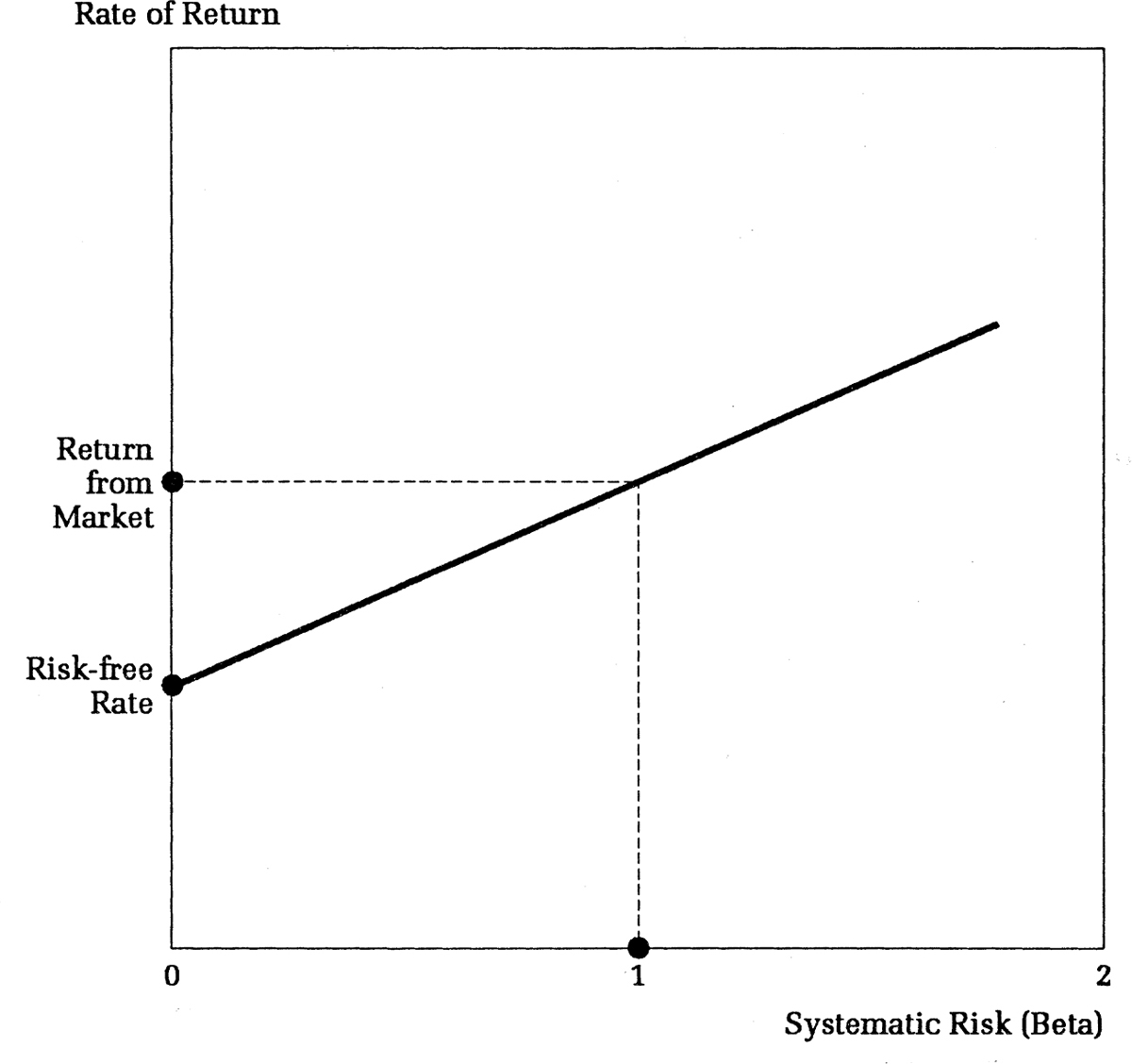
*Those who remember their high school algebra will recall that any straight line can be written as an equation. The equation for the straight line in the diagram is:

Rate of Return = Risk-free Rate + Beta (Return from Market – Risk-free Rate).

Alternatively, the equation can be written as an expression for the risk premium, that is, the rate of return on a portfolio of stocks or any individual stock over and above the risk-free rate of interest:

Rate of Return – Risk-free Rate = Beta (Return from Market – Risk-free Rate).

The equation says that the risk premium you get on any stock or portfolio increases directly with the beta value you assume. Some readers may wonder what relationship beta has to the covariance concept that was so critical in our discussion of portfolio theory. The beta for any security is essentially the same thing as the covariance between that security and the market index as measured on the basis of past experience.

ILLUSTRATION OF PORTFOLIO BUILDING*

* Assuming expected market return is 15 percent and risk-free rate is 10 percent.

^† We can also derive the figure for expected return using directly the formula that accompanies the preceding chart:

Rate of Return = 0.10 + ½ (0.15 – 0.10) = 0.125 or 12½%.

Just as stocks had their fads, so beta came into high fashion in the early 1970s. Institutional Investor, the prestigious magazine that spent most of its pages chronicling the accomplishments of professional money managers, put its imprimatur on the movement by featuring on its cover the letter beta on top of a temple and including as its lead story “The Beta Cult! The New Way to Measure Risk.” The magazine noted that money men whose mathematics hardly went beyond long division were now “tossing betas around with the abandon of PhDs in statistical theory.” Even the SEC gave beta its approval as a risk measure in its Institutional Investors Study Report.

On Wall Street, the early beta fans boasted that they could earn higher long-run rates of return simply by buying a few high-beta stocks. Those who thought they were able to time the market thought they had an even better idea. They would buy high-beta stocks when they thought the market was going up, switching to low-beta ones when they feared the market might decline. To accommodate the enthusiasm for this new investment idea, beta measurement services proliferated among brokers, and it was a symbol of progressiveness for an investment house to provide its own beta estimates. Today, you can obtain beta estimates from brokers such as Merrill Lynch and investment advisory services such as Value Line and Morningstar. The beta boosters on the Street oversold their product with an abandon that would have shocked even the most enthusiastic academic scribblers intent on spreading the beta gospel.

LET’S LOOK AT THE RECORD

In Shakespeare’s Henry IV, Part I, Glendower boasts to Hotspur, “I can call spirits from the vasty deep.” “Why, so can I, or so can any man,” says Hotspur, unimpressed. “But will they come when you do call for them?” Anyone can theorize about how security markets work. CAPM is just another theory. The really important question is: Does it work?

Certainly many institutional investors have embraced the beta concept. Beta is, after all, an academic creation. What could be more staid? Simply created as a number that describes a stock’s risk, it appears almost sterile in nature. The closet chartists love it. Even if you don’t believe in beta, you have to speak its language because, back on the nation’s campuses, my colleagues and I have been producing a long line of PhDs and MBAs who spout its terminology. They now use beta as a method of evaluating a portfolio manager’s performance. If the realized return is larger than that predicted by the portfolio beta, the manager is said to have produced a positive alpha. Lots of money in the market sought out managers who could deliver the largest alpha.

But is beta a useful measure of risk? Is it true that high-beta portfolios will provide larger long-term returns than lower-beta ones, as the capital-asset pricing model suggests? Does beta alone summarize a security’s total systematic risk, or do we need to consider other factors as well? In short, does beta really deserve an alpha? These are subjects of intense current debate among practitioners and academics.

In a study published in 1992, Eugene Fama and Kenneth French divided all traded stocks into deciles according to their beta measures over the 1963–90 period. Decile 1 contained the 10 percent of all stocks that had the lowest betas; decile 10 contained the 10 percent that had the highest betas. The remarkable result, shown in the chart below, is that there was essentially no relationship between the return of these decile portfolios and their beta measures. I found a similar result for the relationship between return and beta for mutual funds. There was no relationship between returns for stocks or portfolios and their beta risk measures.

AVERAGE MONTHLY RETURN VS. BETA: 1963–90 (FAMA AND FRENCH STUDY)

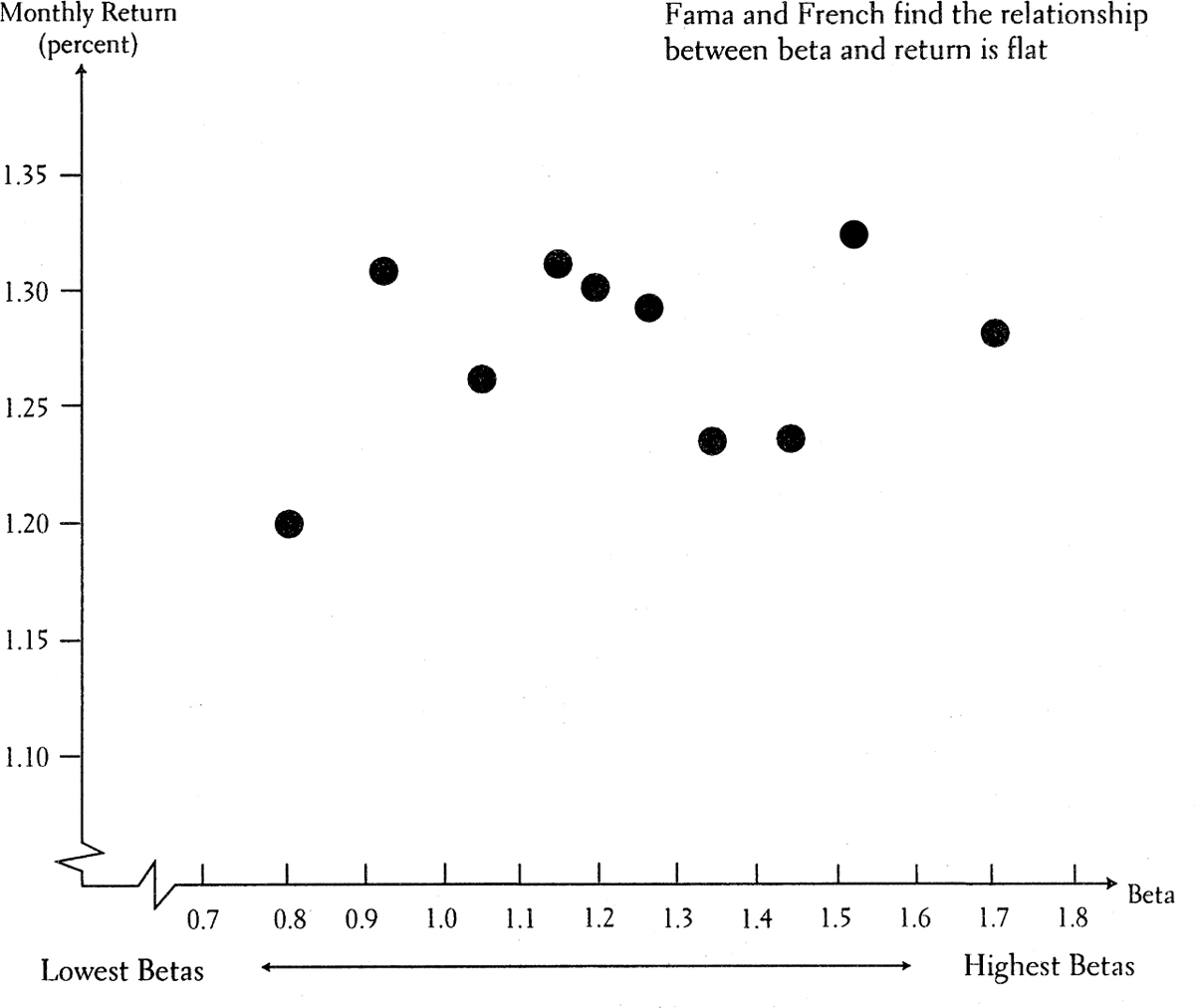
Because their comprehensive study covered a period of almost thirty years, Fama and French concluded that the relationship between beta and return is essentially flat. Beta, the key analytical tool of the capital-asset pricing model, is not a useful single measure to capture the relationship between risk and return. And so, by the mid-1990s, not only practitioners but even many academics as well were ready to assign beta to the scrap heap. The financial press, which earlier had chronicled the ascendancy of beta, now ran feature stories with titles such as “The Death of Beta,” “Bye, Bye Beta,” and “Beta Beaten.” Typical of the times was a letter quoted in Institutional Investor from a writer known only as “Deep Quant.”^† The letter began, “There is a very big story breaking in money management. The Capital-Asset Pricing Model is dead.” The magazine went on to quote one “turncoat quant” as follows: “Advanced mathematics will become to investors what the Titanic was to sailing.” And so the whole set of tools making up the new investment technology—including even modern portfolio theory—came under a cloud of suspicion.

AN APPRAISAL OF THE EVIDENCE

My own guess is that the “turncoat quant” is wrong. The unearthing of serious cracks in the CAPM will not lead to an abandonment of mathematical tools in financial analysis and a return to traditional security analysis. The financial community is not ready to write an obituary for beta at this time. There are many reasons, I believe, to avoid a rush to judgment.

First, it is important to remember that stable returns are preferable, that is, less risky than very volatile returns. Clearly, if one could earn only the same return drilling for oil as from a riskless government security, only those who loved gambling for gambling’s sake alone would drill for oil. If investors really did not worry at all about volatility, the multitrillion-dollar derivative-securities markets would not be thriving as they are. Thus, the beta measure of relative volatility does capture at least some aspects of what we normally think of as risk. And portfolio betas from the past do a reasonably good job of predicting relative volatility in the future.

© Milt Priggee / Pensions & Investments. www.miltpriggee.com. Reprinted by permission.

Second, as Professor Richard Roll of UCLA has argued, we must keep in mind that it is very difficult (indeed probably impossible) to measure beta with any degree of precision. The S&P 500 Index is not “the market.” The total stock market contains many thousands of additional stocks in the United States and thousands more in foreign countries. Moreover, the total market includes bonds, real estate, commodities, and assets of all sorts, including one of the most important assets any of us has—the human capital built up by education, work, and life experiences. Depending on exactly how you measure the “market,” you can obtain very different beta values. One’s conclusions about the capital-asset pricing model and beta as a measure of risk depend very much on how you measure beta. Two economists from the University of Minnesota, Ravi Jagannathan and Zhenyu Wang, find that when the market index (against which we measure beta) is redefined to include human capital and when betas are allowed to vary with cyclical fluctuations in the economy, the support for the CAPM and beta as a predictor of returns is quite strong.

Finally, investors should be aware that even if the long-run relationship between beta and return is flat, beta can still be a useful investment management tool. Were it in fact the case that low-beta stocks will dependably earn rates of return at least as large as those of high-beta stocks (a very big “if” indeed), then beta would be even more valuable as an investment tool than if the capital-asset pricing model held. Investors should scoop up low-beta stocks and earn returns as attractive as for the market as a whole but with much less risk. And investors who do wish to seek higher returns by assuming greater risk should buy and hold low-beta stocks on margin, thereby increasing their risk and returns. We shall see in chapter 11 that some “smart beta” and “risk parity” strategies are designed to execute that exact strategy. What is clear, however, is that beta, as usually measured, is not a substitute for brains and is not a reliable predictor of long-run future returns.

THE QUANT QUEST FOR BETTER MEASURES OF RISK: ARBITRAGE PRICING THEORY

If beta is damaged as an effective quantitative measure of risk, is there anything to take its place? One of the pioneers in the field of risk measurement was Stephen Ross. Ross developed a theory of pricing in the capital markets called arbitrage pricing theory (APT). To understand the logic of APT, one must remember the correct insight underlying the CAPM: The only risk that investors should be compensated for bearing is the risk that cannot be diversified away. Only systematic risk will command a risk premium. But the systematic elements of risk in particular stocks and portfolios may be too complicated to be captured by beta—the tendency of the stocks to move more or less than the market. This is especially so because any particular stock index is an imperfect representative of the general market. Hence, beta may fail to capture a number of important systematic elements of risk.

Let’s take a look at several of these other systematic risk elements. Changes in national income undoubtedly affect returns from individual stocks in a systematic way. This was shown in our illustration of a simple island economy in chapter 8. Also, changes in national income mirror changes in the personal income of individuals, and the systematic relationship between security returns and salary income can be expected to have a significant effect on individual behavior. For example, the laborer in a Ford plant will find that holding Ford common stock is particularly risky, because job layoffs and poor returns from Ford stock are likely to occur at the same time.

Changes in interest rates also systematically affect the returns from individual stocks and are important nondiversifiable risk elements. To the extent that stocks tend to suffer as interest rates go up, equities are a risky investment, and those stocks that are particularly vulnerable to increases in the general level of interest rates are especially risky. Thus, some stocks and fixed-income investments tend to move in parallel, and these stocks will not be helpful in reducing the risk of a bond portfolio. Because fixed-income securities are a major part of the portfolios of many institutional investors, this systematic risk factor is particularly important for some of the largest investors in the market.

Changes in the rate of inflation will similarly tend to have a systematic influence on the returns from common stocks. This is so for at least two reasons. First, an increase in the rate of inflation tends to increase interest rates and thus tends to lower the prices of some equities, as just discussed. Second, the increase in inflation may squeeze profit margins for certain groups of companies—public utilities, for example, which often find that rate increases lag behind increases in costs. On the other hand, inflation may benefit the prices of common stocks in the natural resource industries. Thus, again there are important systematic relationships between stock returns and economic variables that may not be captured adequately by a simple beta measure of risk.

Statistical tests of the influence on security returns of several systematic risk variables have shown somewhat promising results. Better explanations than those given by the CAPM can be obtained for the variation in returns among different securities by using, in addition to the traditional beta measure of risk, a number of systematic risk variables, such as sensitivity to changes in national income, in interest rates, and in the rate of inflation. Of course, the APT measures of risk are beset by some of the same problems faced by the CAPM beta measure.

THE FAMA-FRENCH THREE-FACTOR MODEL

Eugene Fama and Kenneth French have proposed a factor model, like arbitrage pricing theory, to account for risk. Two factors are used in addition to beta to describe risk. The factors derive from their empirical work showing that returns are related to the size of the company (as measured by the market capitalization) and to the relationship of its market price to its book value. Fama-French argue that smaller firms are relatively risky. One explanation might be that they will have more difficulty sustaining themselves during recessionary periods and thus may have more systematic risk relative to fluctuations in GDP. Fama-French also argue that stocks with low market prices relative to their book values may be in some degree of “financial distress.” These views are hotly debated, and not everyone agrees that the Fama-French factors measure risk. But certainly in early 2009, when the stocks of major banks sold at very low prices relative to their book values, it was hard to argue that investors did not consider them in danger of going bankrupt. And even those who would argue that low-market-to-book-value stocks provide higher returns because of investor irrationality find the Fama-French risk factors useful.

THE FAMA-FRENCH RISK FACTORS

A MULTIFACTOR EXPLANATION OF STOCK PRICES

The Fama-French insights generated an even broader set of factors that can be used to explain differential stock returns and that might be used to build investment strategies. For example, highly profitable companies with persistent profit margins have tended to be successful companies in the future. Associated with “profitability” is a so-called “quality” factor, encompassing stable earnings and low operating and financial leverage. While neither profitability nor quality can be considered measures of risk, they both are powerful predictors of the cross section of equity returns. Another very useful factor has been momentum: the tendency for relatively strong stocks to continue to produce good returns. While several other factors have been suggested, almost all of the differences in the returns of diversified portfolios can be explained by the factors described above. Factor models are used extensively now to measure investment performance and to design “smart beta” portfolios, as will be discussed in chapter 11.

A SUMMING UP

Chapters 8 and 9 have been an academic exercise in the modern theory of capital markets. The stock market appears to be an efficient mechanism that adjusts quite quickly to new information. Neither technical analysis, which analyzes the past price movements of stocks, nor fundamental analysis, which analyzes more basic information about the prospects for individual companies and the economy, seems to yield consistent benefits. It appears that the only way to obtain higher long-run investment returns is to accept greater risks.

Unfortunately, a perfect risk measure does not exist. Beta, the risk measure from the capital-asset pricing model, looks nice on the surface. It is a simple, easy-to-understand measure of market sensitivity. Alas, beta also has its warts. The actual relationship between beta and rate of return has not corresponded to the relationship predicted in theory during long periods of the twentieth century. Moreover, betas for individual stocks are not stable over time, and they are very sensitive to the market proxy against which they are measured.

I have argued here that no single measure is likely to capture adequately the variety of systematic risk influences on individual stocks and portfolios. Returns are probably sensitive to general market swings, to changes in interest and inflation rates, to changes in national income, and, undoubtedly, to other economic factors such as exchange rates. Moreover, there is evidence that returns are higher for stocks with lower price-book ratios and smaller size. Other factors such as profitability and momentum also appear to play a role. The mystical perfect risk measure is still beyond our grasp.

To the great relief of assistant professors who must publish or perish, there is still much debate within the academic community on risk measurement, and much more empirical testing needs to be done. Undoubtedly, there will yet be many improvements in the techniques of risk analysis, and the quantitative analysis of risk measurement is far from dead. My own guess is that future risk and factor measures will be even more sophisticated—not less so. Nevertheless, we must be careful not to accept beta or any other measure as an easy way to assess risk and to predict future returns with any certainty. You should know about the best of the modern techniques of the new investment technology—they can be useful aids. But there is never going to be a handsome genie who will appear and solve all our investment problems. And even if he did, we would probably foul it up—as did the little old lady in the following favorite story of Robert Kirby of Capital Guardian Trust:

*In general, the beta of a portfolio is simply the weighted average of the betas of its component parts.

†“Quant” is the Wall Street nickname for the quantitatively inclined financial analyst who devotes attention largely to the new investment technology.