8

A NEW WALKING SHOE: MODERN PORTFOLIO THEORY

. . . Practical men, who believe themselves to be quite exempt from any intellectual influence, are usually the slaves of some defunct economist. Madmen in authority, who hear voices in the air, are distilling their frenzy from some academic scribbler of a few years back.

—J. M. Keynes, The General Theory of Employment, Interest and Money

THROUGHOUT THIS BOOK, I have attempted to explain the theories used by professionals—simplified as the firm-foundation and the castle-in-the-air theories—to predict the valuation of stocks. As we have seen, many academics have earned their reputations by attacking these theories and maintaining that they cannot be relied on to yield extraordinary profits.

As graduate schools continued to grind out bright young financial economists, the attacking academics became so numerous that it seemed obvious that a new strategy was needed; ergo, the academic community busily went about erecting its own theories of stock-market valuation. That’s what this part of the book is all about: the rarefied world of the “new investment technology” created within the towers of the academy. One insight—modern portfolio theory (MPT)—is so basic that it is now widely followed on the Street. The others remain controversial enough to continue to generate thesis material for students and hefty lecture fees for their advisers.

This chapter is about modern portfolio theory, whose insights will enable you to reduce risk while possibly earning a higher return. In chapter 9, I turn to the academics who have suggested that investors can increase their returns by assuming a certain kind of risk. Then, in chapters 10 and 11, I cover the arguments of some academics and practitioners who conclude that psychology, not rationality, rules the market, and that there is no such thing as a random walk. They argue that markets are not efficient and that a number of investment strategies can be followed to improve investment results. These include a number of “smart beta” and “risk parity” strategies that have become popular on Wall Street as well as the view that by investing in socially responsible companies you can do good and do well financially at the same time. Then I conclude by showing that, despite all the critics, traditional index funds remain the undisputed champions in taking the most profitable stroll through the market and that they should constitute the core of all portfolios.

THE ROLE OF RISK

The efficient-market hypothesis explains why the random walk is possible. It holds that the stock market is so good at adjusting to new information that no one can predict its future course in a superior manner. Because of the actions of the pros, the prices of individual stocks quickly reflect all the news that is available. Thus, the odds of selecting superior stocks or anticipating the general direction of the market are even. Your guess is as good as that of the ape, your stockbroker, or even mine.

Hmmm. “I smell a rat,” as Samuel Butler wrote long ago. Money is being made in the market; some stocks do outperform others. Some people can and do beat the market. It’s not all chance. Many academics agree; but the method of beating the market, they say, is not to exercise superior clairvoyance but rather to assume greater risk. Risk, and risk alone, determines the degree to which returns will be above or below average.

DEFINING RISK: THE DISPERSION OF RETURNS

Risk is a most slippery and elusive concept. It’s hard for investors—let alone economists—to agree on a precise definition. The American Heritage Dictionary defines risk as “the possibility of suffering harm or loss.” If I am able to buy one-year Treasury bills to yield 2 percent and hold them until they mature, I am virtually certain of earning a 2 percent monetary return, before income taxes. The possibility of loss is so small as to be considered nonexistent. If I hold common stock in my local electric utility for one year, anticipating a 5 percent dividend return, the possibility of loss is greater. The dividend of the company may be cut and, more important, the market price at the end of the year may be much lower, causing me to suffer a net loss. Investment risk, then, is the chance that expected security returns will not materialize and, in particular, that the securities you hold will fall in price.

Once academics accepted the idea that risk for investors is related to the chance of disappointment in achieving expected security returns, a natural measure suggested itself—the probable dispersion of future returns. Thus, financial risk has generally been defined as the variance or standard deviation of returns. Being long-winded, we use the accompanying exhibit to illustrate what we mean. A security whose returns are not likely to depart much, if at all, from its average (or expected) return is said to carry little or no risk. A security whose returns from year to year are likely to be quite volatile (and for which sharp losses occur in some years) is said to be risky.

Illustration: Expected Return and Variance Measures of Reward and Risk

This simple example will illustrate the concept of expected return and variance and how these are measured. Suppose you buy a stock from which you expect the following overall returns (including both dividends and price changes) under different economic conditions:

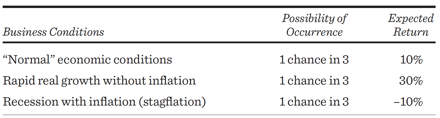
If, on average, a third of past years have been “normal,” another third characterized by rapid growth without inflation, and the remaining third characterized by “stagflation,” it might be reasonable to take these relative frequencies of past events and treat them as our best guesses (probabilities) of the likelihood of future business conditions. We could then say that an investor’s expected return is 10 percent. One-third of the time the investor gets 30 percent, another one-third 10 percent, and the rest of the time she suffers a 10 percent loss. This means that, on average, her yearly return will turn out to be 10 percent.

Expected return = ⅓(0.30) + ⅓(0.10) + ⅓(–0.10) = 0.10.

The yearly returns will be quite variable, however, ranging from a 30 percent gain to a 10 percent loss. The “variance” is a measure of the dispersion of returns. It is defined as the average squared deviation of each possible return from its average (or expected) value, which we just saw was 10 percent.

Variance = ⅓(0.30–0.10)² + ⅓(0.10–0.10)² + ⅓(–0.10–0.10)²= ⅓(0.20)² + ⅓(0.00)² + ⅓(–0.20)² = 0.0267.

The square root of the variance is known as the standard deviation. In this example, the standard deviation equals 0.1634.

Dispersion measures of risk such as variance and standard deviation have failed to satisfy everyone. “Surely riskiness is not related to variance itself,” the critics say. “If the dispersion results from happy surprises—that is, from outcomes turning out better than expected—no investors in their right minds would call that risk.”

It is, of course, quite true that only the possibility of downward disappointments constitutes risk. Nevertheless, as a practical matter, as long as the distribution of returns is symmetric—that is, as long as the chances of extraordinary gain are roughly the same as the probabilities for disappointing returns and losses—a dispersion or variance measure will suffice as a risk measure. The greater the dispersion or variance, the greater the possibilities for disappointment.

DISTRIBUTION OF MONTHLY RETURNS FOR A PORTFOLIO INVESTED IN THE S&P 500-STOCK INDEX, JANUARY 1970–MARCH 2020

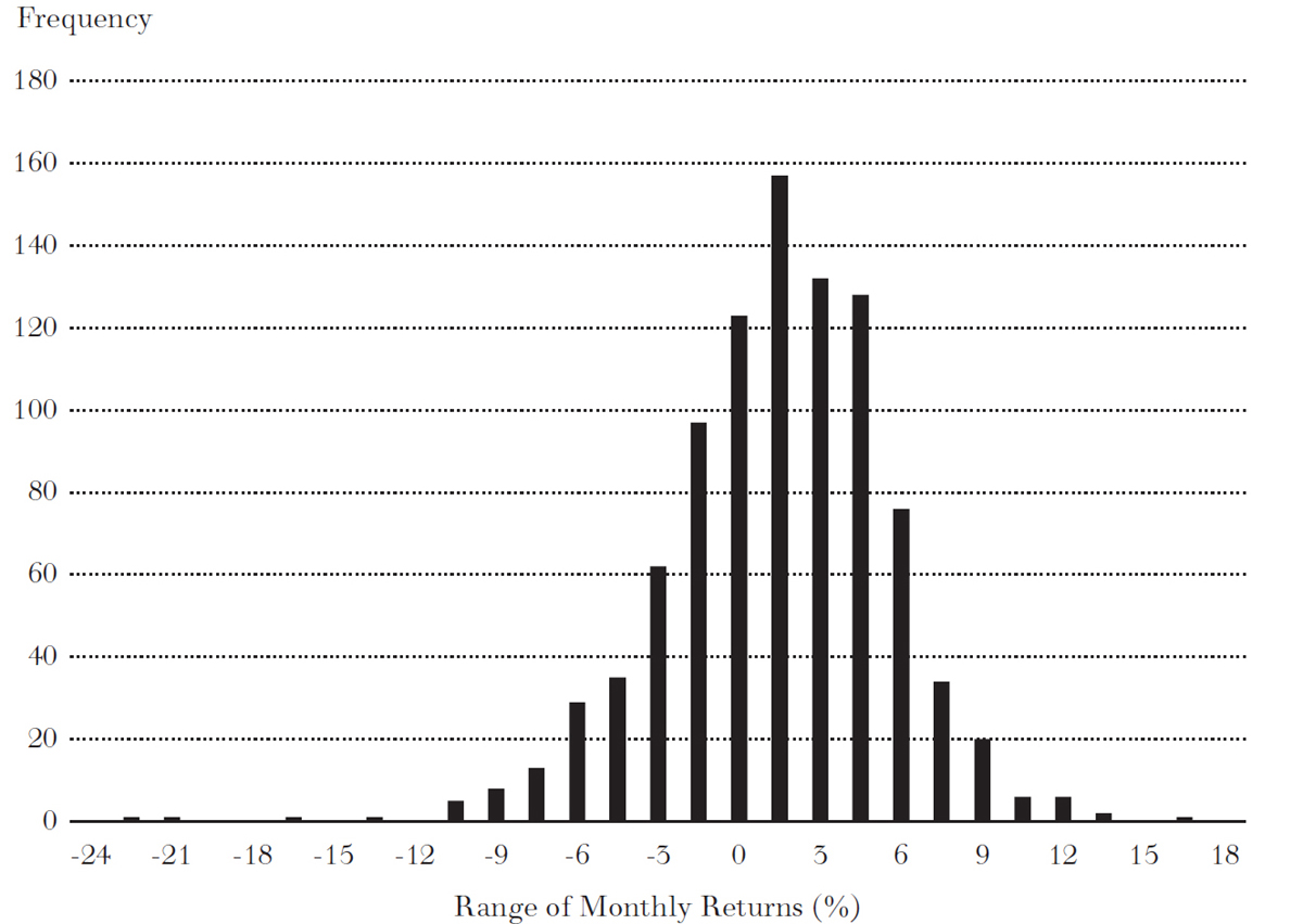
Source: Bloomberg.

Although the pattern of historical returns from individual securities has not usually been symmetric, the returns from well-diversified portfolios of stocks are at least roughly symmetric. The preceding chart shows the distribution of monthly security returns for a portfolio invested in the S&P 500-Stock Index over fifty years. It was constructed by dividing the range of returns into equal intervals (of approximately 1¼ percent) and then noting the frequency (the number of months) with which the returns fell within each interval. On average, the portfolio returned close to 1 percent per month or about 11 percent per year. In periods when the market declined sharply, however, the portfolio also plunged, losing more than 20 percent in a single month.

For reasonably symmetric distributions such as this one, a helpful rule of thumb is that two-thirds of the monthly returns tend to fall within one standard deviation of the average return and 95 percent of the returns fall within two standard deviations. Recall that the average return for this distribution was close to 1 percent per month. The standard deviation (our measure of portfolio risk) turns out to be about 4½ percent per month. Thus, in two-thirds of the months the returns from this portfolio were between +5½ percent and –3½ percent, and 95 percent of the returns were between 10 percent and –8 percent. Obviously, the higher the standard deviation (the more spread out the returns), the more probable it is (the greater the risk) that at least in some periods you will lose money in the market. That’s why a measure of variability such as standard deviation is used and justified as an indication of risk.

DOCUMENTING RISK: A LONG-RUN STUDY

One of the best-documented propositions in the field of finance is that, on average, investors have received higher rates of return for bearing greater risk. The most thorough study has been done by examining data covering the period 1926 through 2020, and the results are shown in the following table. The study took several different investment vehicles—stocks, bonds, and Treasury bills—and measured the percentage increase or decrease each year for each item. A rectangle or bar was then erected on the baseline to indicate the number of years the returns fell between 0 and 5 percent; another rectangle indicated the number of years the returns fell between 5 and 10 percent; and so on, for both positive and negative returns. The result is a series of bars showing the dispersion of returns and from which the standard deviation can be calculated.

BASIC SERIES: SUMMARY STATISTICS OF ANNUAL TOTAL RETURNS FROM 1926 to 2020

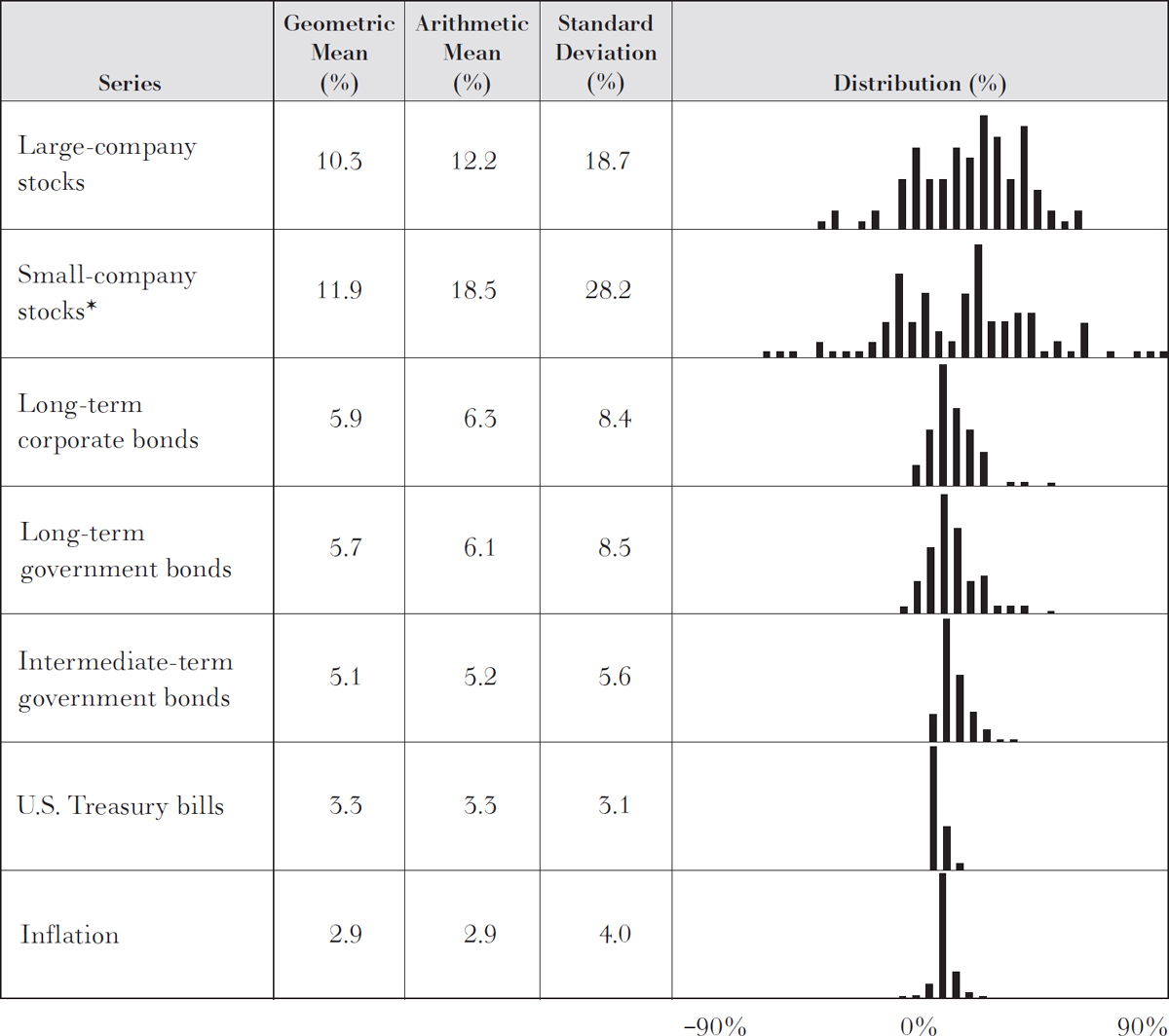
*The 1933 Small-Company Stocks Total Return was 142.9 percent.

Source: Ibbotson, Duff & Phelps SBBI Yearbook.

A quick glance shows that over long periods of time, common stocks have, on average, provided relatively generous total rates of return. These returns, including dividends and capital gains, have exceeded by a substantial margin the returns from long-term bonds, Treasury bills, and the inflation rate as measured by the annual rate of increase in consumer prices. Thus, stocks have tended to provide positive “real” rates of return, that is, returns after washing out the effects of inflation. The long run data show, however, that common-stock returns are highly variable, as indicated by the standard deviation and the range of annual returns, shown in adjacent columns of the table. Returns from equities have ranged from a gain of more than 50 percent (in 1933) to a loss of almost the same percentage (in 1931). Clearly, the extra returns that have been available to investors from stocks have come at the expense of assuming considerably higher risk. Note that small-company stocks have provided an even higher rate of return since 1926, but the dispersion (standard deviation) of those returns has been even larger than for equities in general. Again, we see that higher returns are associated with higher risks.

Investors have suffered through a number of periods when common stocks have produced negative rates of return. The period 1930–32 was extremely poor for stock-market investors. The early 1970s also produced negative returns. The one-third decline in the broad stock-market averages during October 1987 is the most dramatic change in stock prices during a brief period since the 1930s. And stock investors know only too well how poorly stocks performed during the first decade of the 2000s and at the onset of the COVID-19 pandemic in 2020. Still, over the long haul, investors have been rewarded with higher returns for taking on more risk. However, there are ways in which investors can reduce risk. This brings us to the subject of modern portfolio theory, which has revolutionized the investment thinking of professionals.

REDUCING RISK: MODERN PORTFOLIO THEORY (MPT)

Portfolio theory begins with the premise that all investors are like my wife—they are risk-averse. They want high returns and guaranteed outcomes. The theory tells investors how to combine stocks in their portfolios to give them the least risk possible, consistent with the return they seek. It also gives a rigorous mathematical justification for the time-honored investment maxim that diversification is a sensible strategy for individuals who like to reduce their risk.

The theory was developed in the 1950s by Harry Markowitz, and for his contribution he was awarded the Nobel Prize in Economics in 1990. His book Portfolio Selection was an outgrowth of his PhD dissertation at the University of Chicago. His experience has ranged from teaching at UCLA to designing a computer language at RAND Corporation. He even ran a hedge fund. What Markowitz discovered was that portfolios of risky (volatile) stocks might be put together in such a way that the portfolio as a whole could be less risky than the individual stocks in it.

The mathematics of modern portfolio theory (also known as MPT) is recondite and forbidding; it fills the journals and, incidentally, keeps a lot of academics busy. That in itself is no small accomplishment. Fortunately, there is no need to lead you through the labyrinth of quadratic programming to understand the core of the theory. A single illustration makes the whole game clear.

Let’s suppose we have an island economy with only two businesses. The first is a large resort with beaches, tennis courts, and a golf course. The second is a manufacturer of umbrellas. Weather affects the fortunes of both. During sunny seasons, the resort does a booming business and umbrella sales plummet. During rainy seasons, the resort owner does poorly, while the umbrella manufacturer enjoys high profits. The table below shows hypothetical returns for the two businesses during the different seasons:

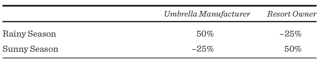
Suppose that, on average, half of the seasons are sunny and half are rainy (i.e., the probability of a sunny or rainy season is ½). An investor who bought stock in the umbrella manufacturer would find that half the time he earned a 50 percent return and half the time he lost 25 percent of his investment. On average, he would earn a return of 12½ percent. This is what we have called the investor’s expected return. Similarly, investment in the resort would produce the same results. Investing in either one of these businesses would be risky, however, because the results are variable and there could be several sunny or rainy seasons in a row.

Suppose, however, that instead of buying only one security, an investor with two dollars diversified and put half his money in the umbrella manufacturer’s and half in the resort owner’s business. In sunny seasons, a one-dollar investment in the resort would produce a 50-cent return, whereas a one-dollar investment in the umbrella manufacturer would lose 25 cents. The investor’s total return would be 25 cents (50 cents minus 25 cents), which is 12½ percent of his total investment of two dollars.

Note that during rainy seasons, exactly the same thing happens—only the names are changed. Investment in the umbrella manufacturer produces a 50 percent return, while the investment in the resort loses 25 percent. Again, the diversified investor makes a 12½ percent return on his total investment.

This simple illustration points out the basic advantage of diversification. Whatever happens to the weather, and thus to the island economy, by diversifying investments over both of the firms, an investor is sure of making a 12½ percent return each year. The trick that made the game work was that although both companies were risky (returns were variable from year to year), the companies were affected differently by weather conditions. (In statistical terms, the two companies had a negative covariance.)^* As long as there is some lack of parallelism in the fortunes of the individual companies in the economy, diversification can reduce risk. In the present case, where there is a perfect negative relationship between the companies’ fortunes (one always does well when the other does poorly), diversification can totally eliminate risk.

Of course, there’s always a rub, and in this case it’s that the fortunes of most companies move pretty much in tandem. When there is a recession and people are unemployed, they may buy neither summer vacations nor umbrellas. Therefore, don’t expect in practice to get the total risk elimination just shown. Nevertheless, because company fortunes don’t always move completely in parallel, investment in a diversified portfolio of stocks is likely to be less risky than investment in one or two single securities.

It is easy to carry the lessons of this illustration to actual portfolio construction. Suppose you were considering combining Ford Motor Company and its major supplier of new tires in a stock portfolio. Would diversification be likely to give you much risk reduction? Probably not. If Ford’s sales slump, Ford will be buying fewer new tires from the tire manufacturer. In general, diversification will not help much if there is a high covariance (high correlation) between the returns of the two companies.

On the other hand, if Ford was combined with a government contractor in a depressed area, diversification might reduce risk substantially. If consumer spending is down, Ford’s sales and earnings are likely to be down and the nation’s level of unemployment up. If the government makes a habit during times of high unemployment of giving out contracts to the depressed area (to alleviate some of the unemployment miseries there), it could well be that the returns of Ford and those of the contractor do not move in phase. The two stocks might have very little covariance or, better still, negative covariance.

The example may seem a bit strained, and most investors will realize that when the market gets clobbered, just about all stocks go down. Still, at least at certain times, some stocks and some classes of assets do move against the market; that is, they have negative covariance or (and this is the same thing) they are negatively correlated with each other.

THE CORRELATION COEFFICIENT AND THE ABILITY OF DIVERSIFICATION TO REDUCE RISK

Now comes the real kicker; negative correlation is not necessary to achieve the risk reduction benefits from diversification. Markowitz’s great contribution to investors’ wallets was his demonstration that anything less than perfect positive correlation can potentially reduce risk. His research led to the results presented in the preceding table. As shown, it demonstrates the crucial role of the correlation coefficient in determining whether adding a security or an asset class can reduce risk.

DIVERSIFICATION IN PRACTICE

To paraphrase Shakespeare, can there be too much of a good thing? In other words, is there a point at which diversification is no longer a magic wand safeguarding returns? Numerous studies have demonstrated that the answer is yes. As shown in the following chart, the golden number for American xenophobes—those fearful of looking beyond our national borders—is at least fifty equal-sized and well-diversified U.S. stocks (clearly, fifty oil stocks or fifty electric utilities would not produce an equivalent amount of risk reduction). With such a portfolio, the total risk is reduced by over 60 percent. And that’s where the good news stops, as further increases in the number of holdings do not produce much additional risk reduction.

THE BENEFITS OF DIVERSIFICATION

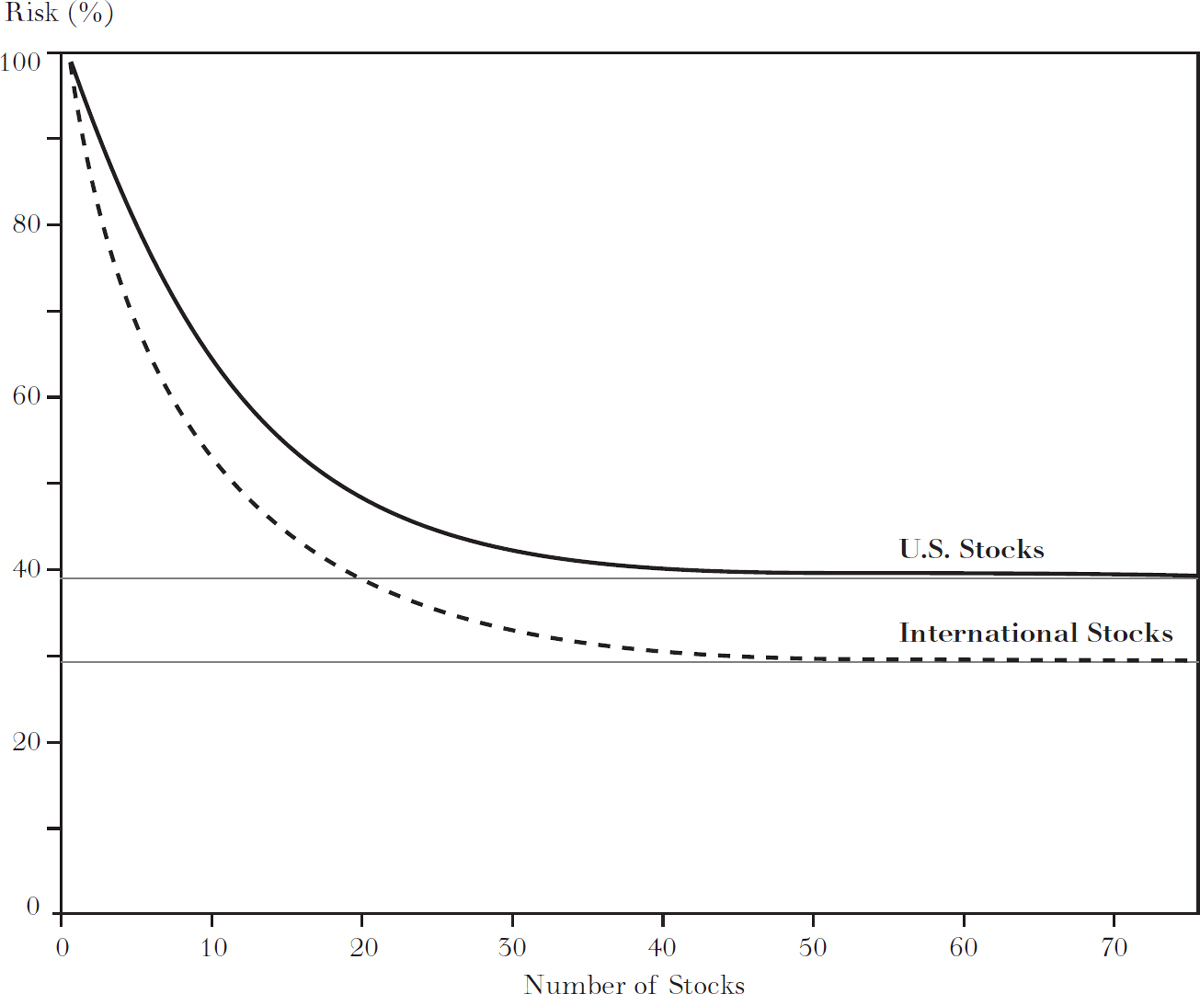
Those with a broader view—investors who recognize that the world has changed considerably since Markowitz first enunciated his theory—can reap even greater protection because the movement of foreign economies is not always synchronous with that of the U.S. economy, especially those in emerging markets. For example, increases in the price of oil and raw materials have a negative effect on Europe, Japan, and even the United States, which is self-sufficient. On the other hand, oil price increases have a very positive effect on Indonesia and oil-producing countries in the Middle East. Similarly, increases in mineral and other raw-material prices have positive effects on nations rich in natural resources such as Australia and Brazil.

It turns out that about fifty is also the golden number for global-minded investors. Such investors get more protection for their money, as shown in the preceding chart. Here, the stocks are drawn not simply from the U.S. stock market but from the international markets as well. As expected, the international diversified portfolio tends to be less risky than the one drawn purely from U.S. stocks.

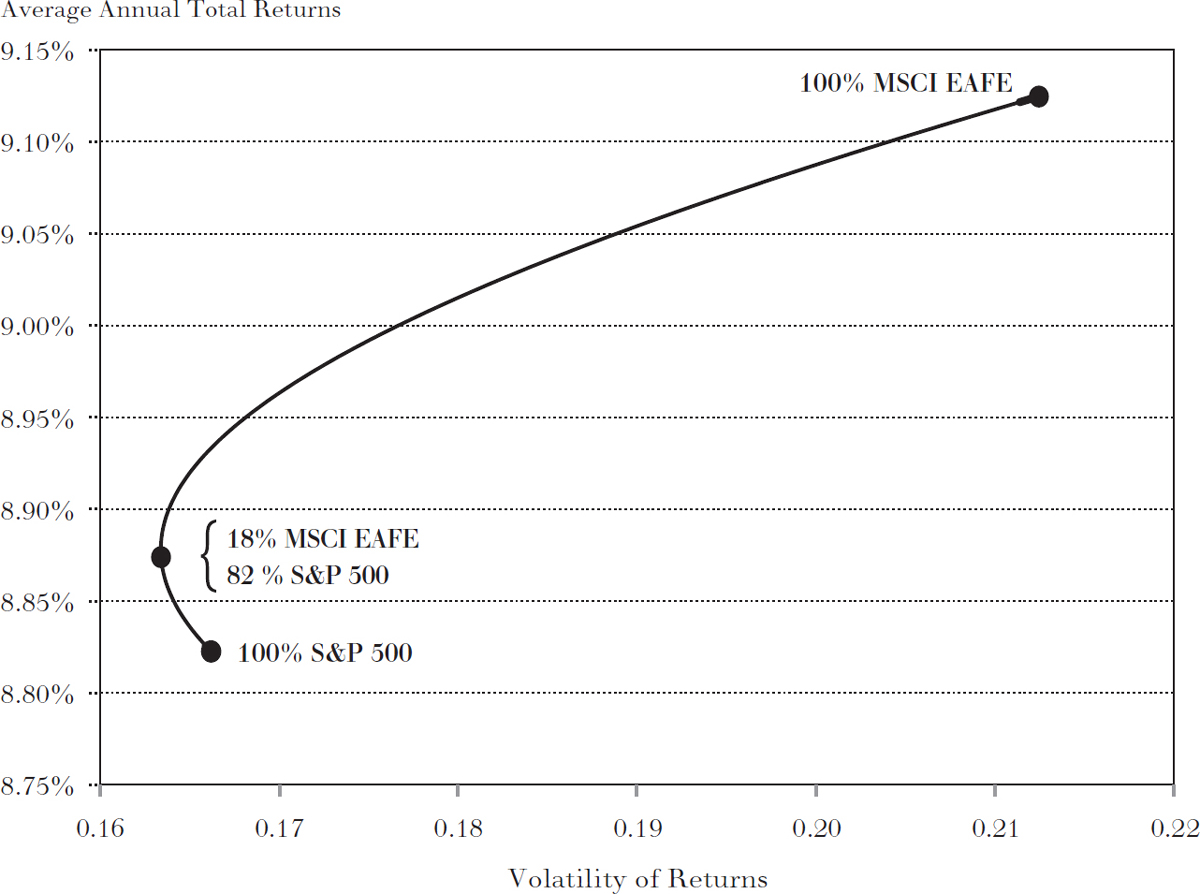
The benefits of international diversification have been well documented. The figure on page 201 shows the gains realized over the more than fifty-year period from 1970. During this time period, foreign stocks (as measured by the MSCI EAFE [Europe, Australasia, and Far East] Index of developed foreign countries) had an average annual return that was slightly higher than the U.S. stocks in the S&P 500 Index. U.S. stocks, however, were safer in that their year-to-year returns were less volatile. The correlation between the returns from the two indexes during this time period was around 0.5—positive but only moderately high. The figure shows the different combinations of return and risk (volatility) that could have been achieved if an investor had held different combinations of U.S. and EAFE (developed foreign country) stocks. At the right-hand side of the figure, we see the higher return and higher risk level (greater volatility) that would have been achieved with a portfolio of only EAFE stocks. At the left-hand side of the figure, the return and risk level of a totally domestic portfolio of U.S. stocks are shown. The solid dark line indicates the different combinations of return and volatility that would result from different portfolio allocations between domestic and foreign stocks.

Note that as the portfolio shifts from a 100 percent domestic allocation to one with gradual additions of foreign stocks, the return tends to increase because EAFE stocks produced a slightly higher return than domestic stocks over this period. The significant point, however, is that adding some of these riskier securities actually reduces the portfolio’s risk level—at least for a while. Eventually, however, as larger and larger proportions of the riskier EAFE stocks are put into the portfolio, the overall risk rises with the overall return.

DIVERSIFICATION OF U.S. AND DEVELOPED FOREIGN COUNTRY STOCKS, JANUARY 1970–DECEMBER 2019

Source: Bloomberg.

The paradoxical result of this analysis is that overall portfolio risk is reduced by the addition of a small amount of riskier foreign securities. Good returns from Japanese automakers balanced out poor returns from domestic ones when the Japanese share of the U.S. market increased. On the other hand, good returns from U.S. manufacturers offset poor returns from foreign manufacturers when the dollar became more competitive and Japan and Europe remained in a recession as the U.S. economy boomed. It is precisely these offsetting movements that reduced the overall volatility of the portfolio.

It turns out that the portfolio with the least risk had 18 percent foreign securities and 82 percent U.S. securities. Moreover, adding 18 percent EAFE stocks to a domestic portfolio also tended to increase the portfolio return. International diversification provided the closest thing to a free lunch available in our world securities markets. When higher returns can be achieved with lower risk by adding international stocks, no investor should fail to take notice.

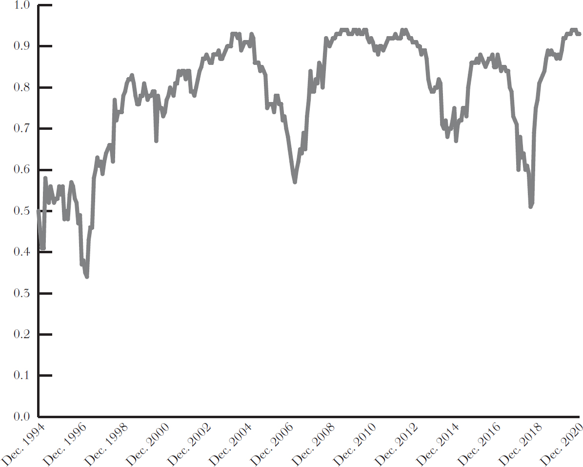
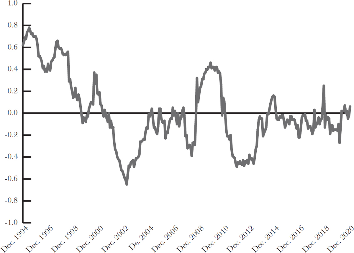
Some portfolio managers have argued that diversification has not continued to give the same degree of benefit as was previously the case. Globalization led to an increase in the correlation coefficients between the U.S. and foreign markets as well as between stocks and commodities. The following chart indicates how correlation coefficients have risen over the first decades of the 2000s. The chart shows the correlation coefficients calculated over every twenty-four-month period between U.S. stocks (as measured by the S&P 500-Stock Index) and the EAFE index of developed foreign stocks. Particularly upsetting for investors is that correlations have been especially high when markets have been falling. During the global credit crisis of 2007–09, all markets fell in unison. The same was true in early 2020 when the COVID-19 pandemic spread rapidly throughout the world. There was apparently no place to hide. Small wonder that some investors came to believe that diversification no longer seemed to be as effective a strategy to decrease risk. Portfolio managers like to say that the only thing that rises during a time of financial panic is the correlation coefficient between asset classes.

TWO-YEAR ROLLING CORRELATION BETWEEN S&P 500 AND MSCI EAFE INDEX

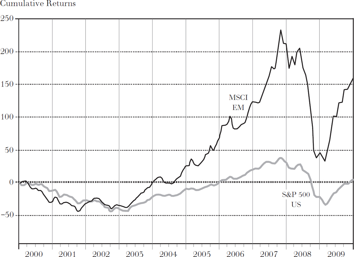
Correlations have risen over time although to a somewhat lesser extent between the U.S. stock market and the MSCI emerging markets index as well as between stocks and the Goldman Sachs (GSCI) index of commodities, such as oil, metals, and the like. But even though correlations between markets have risen, they are still far from perfectly correlated, and broad diversification will still tend to reduce the volatility of a portfolio. And even over periods when different equity markets tended to zig and zag together, diversification still provided substantial benefits. Consider the first decade of the twenty-first century, which was widely referred to as a “lost decade” for U.S. equity investors. Markets in developed countries—the United States, Europe, and Japan—ended the decade at or below their levels at the start of the decade. Investors who limited their portfolios to stocks in developed economies failed to earn satisfactory returns. But over that same decade, investors who included equities from emerging markets (which were easily available through low-cost, broadly diversified emerging-market equity index funds) enjoyed quite satisfactory equity investment performance.

The following graph shows that an investment in the S&P 500 did not make any money during the first decade of the 2000s. But investment in a broad emerging-market index produced quite satisfactory returns. Broad international diversification would have been of enormous benefit to U.S. investors, even during “the lost decade.”

DIVERSIFICATION INTO EMERGING MARKETS HELPED DURING “THE LOST DECADE”: CUMULATIVE RETURNS FROM ALTERNATIVE MARKETS

Source: Vanguard, Datastream, Morningstar.

Moreover, safe bonds proved their worth as a risk reducer. The graph on page 205 shows how correlation coefficients between U.S. Treasury bonds and large capitalization U.S. equities fell during the 2008–09 financial crisis. Even during the horrible stock market of 2008, a broadly diversified portfolio of bonds invested in the Barclay’s Capital broad bond index returned 5.2 percent. There was a place to hide during the financial crisis. Bonds (and bond-like securities to be covered in Part Four) have proved their worth as an effective diversifier.

TIME VARYING STOCK–BOND CORRELATION

Source: Vanguard.

In summary, the timeless lessons of diversification are as powerful today as they were in the past. In Part Four, I will rely on portfolio theory to craft appropriate asset allocations for individuals in different age brackets and with different risk tolerances.

*Statisticians use the term “covariance” to measure what I have called the degree of parallelism between the returns of the two securities. If we let R stand for the actual return from the resort and be the expected or average return, whereas U stands for the actual return from the umbrella manufacturer and Ū is the average return, we define the covariance between U and R (or COV_UR) as follows:

COV_UR = Prob. rain (U, if rain − Ū) (R, if rain − ) + Prob. sun (U, if sun− Ū) (R, if sun − ).

From the preceding table of returns and assumed probabilities, we can fill in the relevant numbers:

COV_UR = ½(0.50 – 0.125) (–0.25 – 0.125) + ½(–0.25 – 0.125) (0.50 – 0.125) = –0.141.

Whenever the returns from two securities move in tandem (when one goes up, the other always goes up), the covariance number will be a large positive number. If the returns are completely out of phase, as in the present example, the two securities are said to have negative covariance.